Research article Topical Sections

Smoking dynamics with health education effect

  • This paper provides a mathematical study for analyzing the dynamics of smoking with health education campaigns involved. The method of next generation matrix is used to derive the basic reproduction number R0. We prove that the smoking-free equilibrium is both locally and globally asymptotically stable if R0<1; and the smoking-present equilibrium is globally asymptotically stable if R0>1. By comparing with smoking dynamics without health education involved, we conclude that health education can decrease smoking population. Numerical simulations are used to support our conclusions.

    Citation: Pengcheng Xiao, Zeyu Zhang, Xianbo Sun. Smoking dynamics with health education effect[J]. AIMS Mathematics, 2018, 3(4): 584-599. doi: 10.3934/Math.2018.4.584

    Related Papers:

    [1] Mehmet Kocabiyik, Mevlüde Yakit Ongun . Construction a distributed order smoking model and its nonstandard finite difference discretization. AIMS Mathematics, 2022, 7(3): 4636-4654. doi: 10.3934/math.2022258
    [2] Cicik Alfiniyah, Wanwha Sonia Putri Artha Soetjianto, Ahmadin, Muhamad Hifzhudin Noor Aziz, Siti Maisharah Sheikh Ghadzi . Mathematical modeling and optimal control of tuberculosis spread among smokers with case detection. AIMS Mathematics, 2024, 9(11): 30472-30492. doi: 10.3934/math.20241471
    [3] Qianqian Cui, Qiang Zhang, Zengyun Hu . Modeling and analysis of Cystic Echinococcosis epidemic model with health education. AIMS Mathematics, 2024, 9(2): 3592-3612. doi: 10.3934/math.2024176
    [4] Peijiang Liu, Taj Munir, Ting Cui, Anwarud Din, Peng Wu . Mathematical assessment of the dynamics of the tobacco smoking model: An application of fractional theory. AIMS Mathematics, 2022, 7(4): 7143-7165. doi: 10.3934/math.2022398
    [5] Yasir Ramzan, Aziz Ullah Awan, Muhammad Ozair, Takasar Hussain, Rahimah Mahat . Innovative strategies for Lassa fever epidemic control: a groundbreaking study. AIMS Mathematics, 2023, 8(12): 30790-30812. doi: 10.3934/math.20231574
    [6] Komal Bansal, Trilok Mathur, Narinderjit Singh Sawaran Singh, Shivi Agarwal . Analysis of illegal drug transmission model using fractional delay differential equations. AIMS Mathematics, 2022, 7(10): 18173-18193. doi: 10.3934/math.20221000
    [7] Sayed Saber, Azza M. Alghamdi, Ghada A. Ahmed, Khulud M. Alshehri . Mathematical Modelling and optimal control of pneumonia disease in sheep and goats in Al-Baha region with cost-effective strategies. AIMS Mathematics, 2022, 7(7): 12011-12049. doi: 10.3934/math.2022669
    [8] Abdul Qadeer Khan, Fakhra Bibi, Saud Fahad Aldosary . Bifurcation analysis and chaos in a discrete Hepatitis B virus model. AIMS Mathematics, 2024, 9(7): 19597-19625. doi: 10.3934/math.2024956
    [9] E. A. Almohaimeed, A. M. Elaiw, A. D. Hobiny . Modeling HTLV-1 and HTLV-2 co-infection dynamics. AIMS Mathematics, 2025, 10(3): 5696-5730. doi: 10.3934/math.2025263
    [10] Hongshuang Wang, Sida Kang, Yuhan Hu . Dynamic analysis and optimal control of rumor propagation models considering different education levels and hesitation mechanisms. AIMS Mathematics, 2024, 9(8): 20089-20117. doi: 10.3934/math.2024979
  • This paper provides a mathematical study for analyzing the dynamics of smoking with health education campaigns involved. The method of next generation matrix is used to derive the basic reproduction number R0. We prove that the smoking-free equilibrium is both locally and globally asymptotically stable if R0<1; and the smoking-present equilibrium is globally asymptotically stable if R0>1. By comparing with smoking dynamics without health education involved, we conclude that health education can decrease smoking population. Numerical simulations are used to support our conclusions.


    1. Introduction

    The smoking behaviors have been considered as a critical problem on both health and social aspects for a long time. It is well-known that smoking can increase the risks of having serious diseases such as cancer and cardiovascular disease. WHO has estimated that tobacco use (smoking and smokeless) is currently responsible for the death of about six million people across the world each year with many of these deaths occurring prematurely. Although often associated with ill-health, disability and death from noncommunicable chronic diseases, tobacco smoking is also associated with an increased risk of death from communicable diseases [1].

    To reduce such serious effect, many nations and global health organizations had applied control policies. According to WHO Comprehensive Information Systems, During the most recent decade, the prevalence of tobacco smoking in men fell in 125 (72%) countries, and in women fell in 155 (87%) countries. If these trends continue, only 37 (21%) countries are on track to achieve their targets for men and 88 (49%) are on track for women, and there would be an estimated 1.1 billion current tobacco smokers (95% credible interval 700 million to 1.6 billion) in 2025 [2]. Among many control policies, health education campaigns played an important role. Ian Bier et al. [3] studied the relationship between auricular acupuncture, education, and smoking cessation. They concluded that acupuncture and education, alone and in combination, significantly reduce smoking. Damiende Walque [4] collected data from smoking population, and concluded that education does affect smoking decisions: educated individuals are less likely to smoke, and among those who initiated smoking, they are more likely to have stopped. Moreover, Sarah Durkin et al. [5] directly studied how mass media campaigns to promote smoking cessation among adults. Their studies showed that mass media campaigns conducted in the context of comprehensive tobacco control programmes can promote quitting and reduce adult smoking prevalence. Mass media campaigns to promote quitting are important investments as part of comprehensive tobacco control programmes to educate about the harms of smoking, set the agenda for discussion, change smoking attitudes and beliefs, increase quitting intentions and quit attempts, and reduce adult smoking prevalence.

    Above evidences motivated us to construct a mathematical model to mimic the smoking dynamics with health educational campaigns involved. We think it can be a helpful tool to analyze smoking behaviors and their control.

    Back to 90's, smoking dynamics were only been studied by using basic SIR model. In a recent decade, several more sophisticated models about smoking dynamics have been studied. In 2008, Sharomo and Gumel [6] introduced new classes Qt (temporary quitter) and Qp (permanent quitter) into the model and presented a more realistic dynamics about smoking population. In 2014, Alkhudhari et al. [7] further developed Sharomo and Gumel's model by considering peer pressure effect on the transmission from Qt (temporary quitter) to S (Smoker). Besides, several researchers like Din et al. [8] have studied the effect of introducing the class Z of smoker with illnesses. Similar models about smoking, drinking can also be found in other studies including [9,10,11,12,13,14,15].

    Above works guide us to derive a smoking model along with health educational campaigns involved. The paper is organized as follows. In Section 2, we present the model with health education effect, and prove the model is well posed. Section 3 focuses on the existence of smoking-free equilibrium and smoking-present equilibrium. Derivations for the reproduction number and both local and global stability properties for equilibria are also included in this section. In Section 4, we provide some numerical simulation results to support our analytic results. Section 5 includes discussions of the results.


    2. Model formulation and its properties


    2.1. Formulation of the model

    In this section we describe our smoking model with health educational campaigns involved. We first divide the whole population into 6 groups:

    PN(t): Normal susceptible population, who do not smoke or smoke occasionally and do not get health education, may become smokers in future.PE(t): Educated susceptible population, who get health education and do not smoke or smoke occasionally, have lower chance to develop smoking behaviors.S(t): Smoking populationQt(t): Temporary quitters, who are currently abstaining smoking, but may not succeed.Qp(t): Permanent quitters, who permanently quit smoking, never smoke again.Z(t): Smokers with associated diseases, yield extra death rate.

    The total number of population at time t is given by

    N(t)=PN(t)+PE(t)+S(t)+Qt(t)+Qp(t)+Z(t)

    The following system of ODEs forms our model (Figure 1):

    Figure 1. Transfer diagram of the model.
    ˙PN=qμμPNβPNS˙PE=(1q)μμPEβδPES˙S=(μ+γ+λ)S+βS(PN+δPE)+αQt˙Qt=μQtαQtηQt+γS˙Qp=μQp+ηQt˙Z=λS(μ+ν)Z

    First of all, every group share same death rate μ. For simplicity, we assume the new recruitment rate of the system to be same as the death rate μ. The new population recruited into the system is divided into 2 portions - uneducated and educated. The proportion q(0<q<1) of new recruitment is uneducated portion, and the proportion (1q) is educated portion. Since smoking population cannot be isolated, through peer pressure, we have both educated and uneducated susceptible population transferring to smokers with transmission coefficient β. However, educated people have lower chance to become smokers, hence we assume addition immunity coefficient δ to reflect this effect, where 0<δ<1. Smokers can turn into temporary quitters by getting treatment or self-abstaining, hence we assume γ as the corresponding transmission coefficient. On the other hand, temporary quitters can also relapse, hence we assume α as the corresponding transmission coefficient. There does exist some quitters could abstain smoking permanently. By enough treatment and perseverance, a temporary quitter can become a permanent quitter. For this type of transmission, we assume a transmission coefficient η. We have mentioned in introduction that smoking is highly related to some serious diseases. Therefore, it is reasonable to have a transmission from ordinary smokers to diseased smokers with coefficient λ. In addition, this diseased population yield extra death rate ν.


    2.2. Properties of the model

    Boundedness is one of important properties of a system, and we shall provide it for our system by following lemma.

    Lemma 2.1. If PN(0)>0, PE(0)>0, S(0)>0, Qt(0)>0, Qp(0)>0, Z(0)>0, then the solutions PN(t)0, PE(t)0, S(t)0, Qt(t)0, Qp(t)0, Z(t)0 for all t>0.

    Proof. Suppose above lemma does not hold, then at least one of PN(t), PE(t), S(t), Qt(t), Qp(t), Z(t) is less than 0 for some t's. We have following 6 cases:

    1. There exists a first time t1 such that PN(t1)=0, PN(t1)<0, and PE(t)0, S(t)0, Qt(t)0, Qp(t)0, Z(t)0 for 0tt1. But PN(t1)=qμ0, so this case is impossible.

    2. There exists a first time t2 such that PE(t2)=0, PE(t2)<0, and PN(t)0, S(t)0, Qt(t)0, Qp(t)0, Z(t)0 for 0tt2. But PE(t2)=(1q)μ0, so this case is impossible.

    3. There exists a first time t3 such that S(t3)=0, S(t3)<0, and PN(t)0, PE(t)0, Qt(t)0, Qp(t)0, Z(t)0 for 0tt3. But S(t3)=00, so this case is impossible.

    4. There exists a first time t4 such that Qt(t4)=0, Qt(t4)<0, and PN(t)0, PE(t)0, S(t)0, Qp(t)0, Z(t)0 for 0tt4. But Qt(t4)=γS(t4)0, so this case is impossible.

    5. There exists a first time t5 such that Qp(t5)=0, Qp(t5)<0, and PN(t)0, PE(t)0, S(t)0, Qt(t)0, Z(t)0 for 0tt5. But Qp(t5)=ηQt(t5)0, so this case is impossible.

    6. There exists a first time t6 such that Z(t6)=0, Z(t6)<0, and PN(t)0, PE(t)0, S(t)0, Qt(t)0, Qp(t)0 for 0tt6. But Z(t6)=λS(t6)0, so this case is impossible.

    That shows the contradiction, therefore the lemma has to be true.

    By summing the equations of our system, we find that

    PN+PE+S+Qt+Qp+Z=μ[1(PN+PE+S+Qt+Qp+Z)]νZμ[1(PN+PE+S+Qt+Qp+Z)]

    It follows that PN(t)+PE(t)+S(t)+Qt(t)+Qp(t)+Z(t)1, so the set

    Ω={(PN,PE,S,Qt,Qp,Z)R6+:PN+PE+S+Qt+Qp+Z1}

    is positively invariant for our system. Hence, the global stability of the system will be only considered within set Ω. Also, the whole population has the scaled upper bound 1 in this model, and the number of each population group can be interpreted as the portion of the whole population.


    3. Equilibria and stabilities


    3.1. Equilibria and local stabilities

    By setting the right-hand side of the model to 0, we get following equations:

    PN=qμμ+βSPE=(1q)μμ+βδSS=αQt(μ+γ+η)β(PN+δPE)Qt=γSμ+η+αQp=ημQtZ=λSμ+ν

    We see that the model has a smoking-free equilibrium E0=(PN0,PE0,0,0,0,0), where

    PN0=q       PE0=1q

    The smoking infected compartments are S, Qt, and Z, giving m=3. Since each function in our model represents a direct transfer of individuals, each function is non negative. And if one population group is empty, then there is no transfer of individuals out of that population group. Also, our model assumes that incidence of smoking infection for uninfected population groups is zero, the smoking free subspace is always invariant, and the smoking free equilibrium is stable in the absence of new infection. This indicates that our model satisfies the five conditions in lemma 1 from van den Driessche and Watmough [16]. Let X=(S,Qt,Z,PN,PE,Qp)T, then the model can be rewritten as

    dXdt=F(X)V(X)

    where

    F(X)=(βPNS+βδPES00000)     V(X)=((μ+γ+λ)SαQt(α+μ+η)QtγS(μ+ν)ZλSμPN+βPNSqμμPE+βδPES(1q)μμQpηQt)

    By computing the Jacobian matrices at E0, we got

    DF(E0)=(F3×3000)     DV(E0)=(V3×30J1J2)

    where

    F=(βPN0+βδPE000000000)     V=(μ+γ+λα0γα+μ+η0λ0μ+ν)
    J1=(βPN000βγPE0000η0)     J2=(μ000μ000μ)

    Further, F is non-negative, V is a non-singular 3-matrix and all eigenvalues of J2 have positive real part. Thus, the basic reproduction number of the model can be derived by the method of next generation matrix [16]. And we got the basic reproduction number R0

    R0=ρ(FV1)=β(PN0+δPE0)(μ+η+α)(μ+γ+λ)(μ+η+α)αγ

    By Theorem 2 from van den Driessche and Watmough [16], the local stability of smoking-free equilibrium E0 can be summarized as following:

    Theorem 3.1. The smoking-free equilibrium E0 is locally asymptotically stable for R0<1 and unstable for R0>1.

    Now we look at smoking-present equilibrium E=(PN,PE,S,Qt,Qp,Z). Similarly, by he right-hand side of the model to 0, we get

    PN=qμμ+βSPE=(1q)μμ+βδSQt=γSμ+η+αS[β(PN+δPE)(μ+γ+λ)]+αQt=0

    By substituting Qt into last equation, we have

    S[β(PN+δPE)(μ+γ+λ)]+γSμ+η+α=0 S(β(PN+δPE)(μ+γ+λ)+γμ+η+α)=0

    Since S0,

    β(PN+δPE)(μ+γ+λ)+γμ+η+α=0 PN+δPE=1β((μ+γ+λ)γμ+η+α)

    By substituting PN and PE, we have

    Y(S):=q(μ+βδS)+(1q)δ(μ+βS)(μ+βS)(μ+βδS)(μ+γ+λ)(μ+η+α)αγμβ(μ+η+α)=0

    By taking the derivative of Y(S), we have

    Y(S)=β{β2δ2S2+μS[2βδ2(1q)+2βδq]+μ2[δ2(1q)+q]}(μ+βS)2(μ+βδS)2<0

    Hence, the function Y(S) is decreasing for S>0. In addition, since (μ+βδS)(μ+βS)>(μ+βδS)βS and q(μ+βδS)+(1q)δ(μ+βS)u+βδS, we have

    Y(S)<1βS(μ+γ+λ)(μ+η+α)αγμβ(μ+η+α)

    Thus,

    Y(0)=(μ+γ+λ)(μ+η+α)αγμβ(μ+η+α)(R01)Y(1)<1β(μ+γ+λ)(μ+η+α)αγμβ(μ+η+α)=λ(μ+η+α)+γ(μ+η)μβ(μ+η+α)<0

    If R0>1, by the monotonicity of Y(S), there exist an unique root in (0,1). If R01, there is not root in (0,1). Since the smoking-present equilibrium E lives in the set Ω={(PN,PE,S,Qt,Qp,Z)R6+:PN+PE+S+Qt+Qp+Z1}, following theorem can be established:

    Theorem 3.2. The system always has the smoking-free equilibrium E0. If R0>1, the system has an unique smoking-present equilibrium E, where

    PN=qμμ+βSPE=(1q)μμ+βδSQt=γSμ+η+αQp=ημQtZ=λSμ+ν

    and S is the unique root of Y(S)=0.

    Theorem 3.3. The smoking-present equilibrium E is locally stable, and there is no hopf bifurcation.

    Proof. Since variables Qp and Z do not appears in first four equations of the system, the dynamics of the system is same as the following one:

    ˙PN=qμμPNβPNS˙PE=(1q)μμPEβδPES˙S=(μ+γ+λ)S+βS(PN+δPE)+αQt˙Qt=μQtαQtηQt+γS

    Consider the previous four equations in the original system, we get its Jacobian matrix at the smoking-present equilibrium E,

    J(E)=[βSμ0βPN00μδSμβδPE0βSβδSβ(δPE+PN)μγλα00γμαη].

    R0=1 reveals that

    β(δPE+PN)μγλ=αγα+η+μ.

    Hence, we have

    J(E)=[βSμ0βPN00μδSμβδPE0βSβδSαγα+η+μα00γμαη].

    Our aim is to prove J(E) has no positive or zero-real part eigenvalues. In order to reduce complexity due to multiple parameters, we introduce new variables, which are all positive from the original parameters are positive.

    a11=βS+μ, a13=βPN, a22=μδS+μ, a23=βδPE, a31=Sβ, a32=Sδβ, a44=μ+α+η.

    Even the new variables are not independent, we would like to investigate them in a broader ranges.

    Then, we have

    J(E)=[a110a1300a22a230a31a32αγa44α00γa44].

    J(E)xI=0 gives the eigen-polynomial,

    Ep(x)=a44x4+(a442+(a11+a22)a44+αγ)x3+((a11+a22)a442+(a11a22+a13a31+a23a32)a44+γα(a11+a22))x2+((a11a22+a13a31+a23a32)a442+(a11a23a32+a13a22a31)a44+γa11a22α)x+a442(a11a23a32+a13a22a31).

    All coefficients of Ep(x) are positive, therefore Ep(x) has no non-negative eigenvalues.Suppose Ep(x) has a pair of complex eigenvalues x=a±bi. Let REp(x) and IPp(x) denote the real part and imaginal part of Ep(x). The resultant between REp(x) and IPp(x) respect to b is a polynomial in a with positive coefficients, which has no non-negative roots. Therefore, J(E) could not have complex eigenvalues with positive or zero real part. Hence, the eigenvalues of J(E) are negative or complex with negative real part, therefore, the smoking-present equilibria E is local stable and could not present hopf-bifurcation.


    3.2. Global stability of equilibria

    Theorem 3.4. If R01, the smoking-free equilibrium E0 is globally asymptotically stable.

    Proof. Since variables Qp and Z do not appears in first four equations of the system, the dynamics of the system is same as the following one:

    ˙PN=qμμPNβPNS˙PE=(1q)μμPEβδPES˙S=(μ+γ+λ)S+βS(PN+δPE)+αQt˙Qt=μQtαQtηQt+γS

    By proving the global stability of smoking-free equilibrium ˉE0(PN0,PE0,0,0) of above system, we prove the original one.

    For the smoking-free equilibrium ¯E0, following equations hold:

    qμμPN=0(1q)μμPE=0

    Hence, we can rewrite above system as

    ˙PN=PN[qμ(1PN1PN0)βS]˙PE=PE[(1q)μ(1PE1PE0)βδS]˙S=βS[(PN0+δPE0)+(PNPN0)+δ(PEPE0)]+αQt(μ+γ+λ)S˙Qt=γS(μ+η+α)Qt

    Define the Lyapunov function:

    V1=(PNPN0PN0lnPNPN0)+(PEPE0PE0lnPEPE0)+S+αμ+η+αQt

    By taking the derivative, we have

    V1=(PNPN0)PNPN+(PEPE0)PEPE+S+αμ+η+αQt=(PNPN0)[qμ(1PN1PN0)βS]+(PEPE0)[(1q)μ(1PE1PE0)βδS]+βS[(PN0+δPE0)+(PNPN0)+δ(PEPE0)]+αQt(μ+γ+λ)S+αμ+η+α[γS(μ+η+α)Qt]=(μ+γ+λ)(μ+η+α)αγμ+η+α(R01)S+F(PN,PE)

    , where

    F(PN,PE)=qμ(PNPN0)(1PN1PN0)+(1q)μ(PEPE0)(1PE1PE0)=qμ(2PNPN0PN0PN)+(1q)μ(2PEPE0PE0PE)

    Let x=PNPN0 and y=PEPE0, then

    F(PN,PE)=qμ(2x1x)+(1q)μ(2y1y)=qμ((1)(x1)2x)+(1q)μ((1)(y1)2y)

    It is obvious that F(PN,PE)0 for x,y>0. In particular, F(PN,PE)=0 if and only if PN=PN0 and PE=PE0. Hence, if R01, V1<0 for PNPN0, PEPE0 and S0. Therefore, by Lyapunov stability criterion, the smoking-free equilibrium ˉE0 is globally asymptotically stable, and so is E0.

    Theorem 3.5. If R0>1, the smoking-present equilibrium E is globally asymptotically stable.

    Proof. Similarly, we prove the stability of original smoking-present equilibrium E by proving the stability of ˉE(PN,PE,S,Qt).

    For ˉE, following equations hold:

    qμμPNβPNS=0(1q)μμPEβδPES=0(μ+γ+λ)S+βS(PN+δPE)+αQt=0γSQt(μ+η+α)=0

    Let a=PNPN, b=PEPE, c=SS, and d=QtQt, we have

    a=a[qμPN(1a1)βS(c1)]b=b[(1q)μPE(1b1)βδS(c1)]c=c[βPN(a1)+βδPE(b1)+αQtS(dc1)]d=d[γSQt(cd1)]

    Define the Lyapunov function:

    V2=PN(a1lna)+PE(b1lnb)+S(c1lnc)+αμ+η+αQt(d1lnd)

    By taking the derivative, we have

    V2=PN(a1a)a+PE(b1b)b+S(c1c)c+αμ+η+αQt(d1d)d=(a1)[qμ(1a1)βPNS(c1)]+(b1)[(1q)μ(1b1)βδPES(c1)]+(c1)[βPNS(a1)+βδPES(b1)+αQt(dc1)]+αγSμ+η+α(d1)(cd1)=qμ(a1)(1a1)βPNS(a1)(c1)+(1q)μ(b1)(1b1)βδPES(b1)(c1)+βPNS(c1)(a1)+βδPES(c1)(b1)+αQt(c1)(dc1)+αγSμ+η+α(d1)(cd1)=qμ((a1)2a)+(1q)μ((b1)2b)+αQt(dcdc+1)αγSμ+η+α(cdcd+1)=F(a,b)+G(c,d)

    where

    F(a,b)=qμ((a1)2a)+(1q)μ((b1)2b)G(c,d)=αγSμ+η+α(2cddc)=αγSμ+η+α((cd)2cd)

    It is easy to see that F(a,b)0 for a,b>0. In particular, F(a,b)=0 if and only if PN=PN and PE=PE. Also, G(c,d)0 for c,d>0. In particular, G(c,d)=0 if and only if SS=QtQt. Hence, V2<0 for PNPN, PEPE, SS, and QtQt. Therefore, by byLyapunov stability criterion, the smoking-free equilibrium ˉE is globally asymptotically stable, and so is E.


    4. Numerical simulation

    In this section, we provide some numerical results to support our analytic results from above. For the choices of parameters, some are chosen from medical researches, and others are estimated. The values for normal mortality μ and additional disease death rate ν are provided by McEvoy, John W., et al. [9]. Other parameters are estimated. All the parameter values show in Table 1.

    Table 1. Table of parameter values.
    ParameterMeaningValueSource
    qnon-educated portion of new recruitment rate0.7Estimated for test case
    μnatural death rate and new recruitment rate0.017McEvoy, John W., et al. "Mortality rates in smokers and nonsmokers in the presence or absence of coronary artery calcification." JACC: Cardiovascular Imaging 5.10 (2012): 1037-1045.
    βtransmission coefficient for potential smokers (both non-educated and educated) transfer to smokers (S)0.2/0.7Estimated for test cases
    δimmuity coefficient for educated population (PE) to lower the transfer to smokers (S)0.25Smoking & Tobacco Use.17 Centers for Disease Control and Prevention, Centers for Disease Control and Prevention, 3 Feb. 2017
    γtransmission coefficient for smokers (S) transfer to temporary quitters (Qt)0.554Morbidity and Mortality Weekly Report (MMWR).17 Centers for Disease Control and Prevention, Centers for Disease Control and Prevention, 14 Aug. 2017
    αtransmission coefficient for temporary quitters (Qt) transfer to smokers (S)0.48Morbidity and Mortality Weekly Report (MMWR).17 Centers for Disease Control and Prevention, Centers for Disease Control and Prevention, 14 Aug. 2017
    ηtransmission coefficient for temporary quitters (Qt) transfer to permanent quitters (Qp)0.074Morbidity and Mortality Weekly Report (MMWR).17 Centers for Disease Control and Prevention, Centers for Disease Control and Prevention, 14 Aug. 2017
    λtransmission coefficient for smokers (S) transfer to smokers with diseases (Z)0.4233Smoking & Tobacco Use.17 Centers for Disease Control and Prevention, Centers for Disease Control and Prevention, 3 Feb. 2017
    νextra death rate for smokers with diseases (Z)0.043McEvoy, John W., et al. "Mortality rates in smokers and nonsmokers in the presence or absence of coronary artery calcification." JACC: Cardiovascular Imaging 5.10 (2012): 1037-1045.
     | Show Table
    DownLoad: CSV

    The model is simulated for following different initial values such that PN(0)+PE(0)+S(0)+Qt(0)+Qp(0)+Z(0)=1:

    1. PN(0)=0.8, PE(0)=0.1, S(0)=0.1, Qt(0)=0Qp(0)=0, Z(0)=0.

    2. PN(0)=0.1, PE(0)=0.1, S(0)=0.8, Qt(0)=0Qp(0)=0, Z(0)=0.

    3. PN(0)=0.2, PE(0)=0.2, S(0)=0.2, Qt(0)=0.2Qp(0)=0.2, Z(0)=0.

    4. PN(0)=0.1, PE(0)=0.1, S(0)=0.5, Qt(0)=0Qp(0)=0, Z(0)=0.3.

    For R0<1, Figure 2 shows that the smoking-free equilibrium E0 is globally asymptotically stable. For R0>1, Figure 3 shows that the smoking-present equilibrium E is globally asymptotically stable.

    Figure 2. R0<1, E0 is globally asymptotically stable.
    Figure 3. R0>1, E is globally asymptotically stable.

    5. Discussion

    In this paper, we consider the health education effect on the smoking dynamic model. We have derived the reproduction number (R0) and obtained the following results: when R0<1, smoking-free equilibrium is both locally and globally asymptotically stable. As the educated susceptible population increases, the permanent quitter population also increases. When R0>1, we proved the smoking-present equilibrium is globally asymptotically stable by constructing Lyapunov function. When the ratio of educated susceptible group increases, the permanent quitter group experiences a time frame of oscillation then becomes stable. The results imply that increasing the health education population not only increases the permanent quitter, but also reduce the difficulty of non-smoking work of the area.

    It will be very interesting to consider the time delay in this model, and it will be more realistic and give us more insights into the smoking dynamics, but some complex dynamic behaviors may occur([15,17]).


    Acknowledgments

    The authors would like to thank the generous support from the mathematics department at University of Evansville.


    Conflict of interest

    Authors declare no conflicts of interest in this paper.


    [1] World Health Organization, WHO global report on trends in prevalence of tobacco smoking 2015, World Health Organization, 2015.
    [2] V. Bilano, S. Gilmour, T. Moffet, et al. Global trends and projections for tobacco use, 1990–2025: an analysis of smoking indicators from the WHO Comprehensive Information Systems for Tobacco Control, The Lancet, 385 (2015), 966–976.
    [3] I. D. Bier, J. Wilson, P. Studt, et al. Auricular acupuncture, education, and smoking cessation: a randomized, sham-controlled trial, Am. J. Public Health, 92 (2002), 1642–1647.
    [4] D. de Walque, Does education affect smoking behaviors?: Evidence using the Vietnam draft as an instrument for college education, J. Health Econ., 26 (2007), 877–895.
    [5] S. Durkin, E. Brennan and M. Wakefield, Mass media campaigns to promote smoking cessation among adults: an integrative review, Tob. control, 21 (2012), 127–138.
    [6] O. Sharomi and A. B. Gumel, Curtailing smoking dynamics: a mathematical modeling approach, Appl. Math. Comput., 195 (2008), 475–499.
    [7] Z. Alkhudhari, S. Al-Sheikh and S. Al-Tuwairqi, Global dynamics of a mathematical model on smoking, International Scholarly Research Notices, 2014 (2014), 1–7.
    [8] D. Qamar, O. Muhammad, H. Takasar, et al. Qualitative behavior of a smoking model, Adv. Differ. Equ-NY, 2016 (2016), 96.
    [9] J. W. McEvoy, M. J. Blaha, J. J. Rivera, et al. Mortality rates in smokers and nonsmokers in the presence or absence of coronary artery calcification, JACC-CARDIOVASC IMAG., 5 (2012), 1037–1045.
    [10] G. Zaman, Qualitative behavior of giving up smoking models, B. Malays. Math. Sci. So., 34 (2009), 403–415.
    [11] H. Xiang, N. N. Song and H. F. Huo, Modeling effects of public health educational campaigns on drinking dynamics, J. Biol. Dynam., 10 (2016), 164–178.
    [12] H. Xiang, C. C. Zhu and H. F. Huo, Modelling the effect of immigration on drinking behaviour, J. Biol. Dynam., 11 (2017), 275–298.
    [13] H. F. Huo and C. C. Zhu, Influence of relapse in a giving up smoking model, Abstr. Appl. Anal., 2013 (2013), 1–12.
    [14] H. F. Huo and N. N. Song, Global stability for a binge drinking model with two-stage, Discrete Dyn. Nat. Soc., 2012 (2012), 1–15.
    [15] H. F. Huo, Y. L. Chen and H. Xiang, Stability of a binge drinking model with delay, J. Biol. Dynam., 11 (2017), 210–225.
    [16] P. Van den Driessche and J. Watmough, Reproduction numbers and sub-threshold endemic equilibria for compartmental models of disease transmission, Math. Biosci., 180 (2002), 29–48.
    [17] H. T. Zhao and M. C. Zhao, Global Hopf bifurcation analysis of an susceptible-infective-removed epidemic model incorporating media coverage with time delay, J. Biol. Dynam., 11 (2017), 8–24.
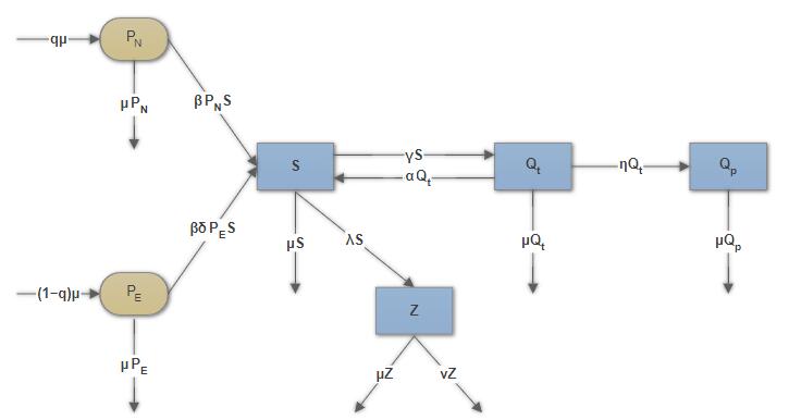
  • This article has been cited by:

    1. Fangfang Yang, Zizhen Zhang, Dynamics of a nonlinear SIQRS computer virus spreading model with two delays, 2021, 6, 2473-6988, 4083, 10.3934/math.2021242
    2. Angdi Zhou, Xinru Li, Yiwen Song, Bingqin Hu, Yitong Chen, Peiyao Cui, Jinghua Li, Academic Performance and Peer or Parental Tobacco Use among Non-Smoking Adolescents: Influence of Smoking Interactions on Intention to Smoke, 2023, 20, 1660-4601, 1048, 10.3390/ijerph20021048
    3. Kottakkaran Sooppy Nisar, Rafia Tabassum, Muhammad Asif Zahoor Raja, Muhammad Shoaib, Advanced Bio-Inspired computing paradigm for nonlinear smoking model, 2023, 76, 11100168, 411, 10.1016/j.aej.2023.06.032
  • Reader Comments
  • © 2018 the Author(s), licensee AIMS Press. This is an open access article distributed under the terms of the Creative Commons Attribution License (http://creativecommons.org/licenses/by/4.0)
通讯作者: 陈斌, bchen63@163.com
  • 1. 

    沈阳化工大学材料科学与工程学院 沈阳 110142

  1. 本站搜索
  2. 百度学术搜索
  3. 万方数据库搜索
  4. CNKI搜索

Metrics

Article views(5925) PDF downloads(799) Cited by(3)

Article outline

Other Articles By Authors

/

DownLoad:  Full-Size Img  PowerPoint
Return
Return

Catalog