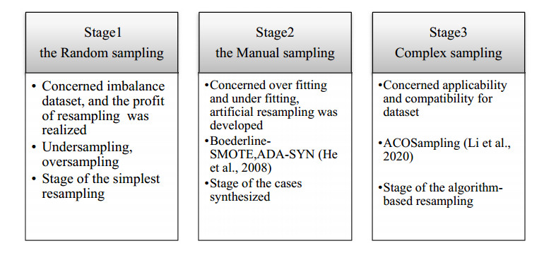
As an important part of machine learning, classification learning has been applied in many practical fields. It is valuable that to discuss class imbalance learning in several fields. In this research, we provide a review of class imbalanced learning methods from the data driven methods and algorithm driven methods based on numerous published papers which studied class imbalance learning. The preliminary analysis shows that class imbalanced learning methods mainly are applied both management and engineering fields. Firstly, we analyze and then summarize resampling methods that are used in different stages. Secondly, we provide a detailed instruction on different algorithms, and then we compare the results of decision tree classifiers based on resampling and empirical cost sensitivity. Finally, some suggestions from the reviewed papers are incorporated with our experiences and judgments to offer further research directions for the class imbalanced learning fields.
Citation: Cui Yin Huang, Hong Liang Dai. Learning from class-imbalanced data: review of data driven methods and algorithm driven methods[J]. Data Science in Finance and Economics, 2021, 1(1): 21-36. doi: 10.3934/DSFE.2021002
As an important part of machine learning, classification learning has been applied in many practical fields. It is valuable that to discuss class imbalance learning in several fields. In this research, we provide a review of class imbalanced learning methods from the data driven methods and algorithm driven methods based on numerous published papers which studied class imbalance learning. The preliminary analysis shows that class imbalanced learning methods mainly are applied both management and engineering fields. Firstly, we analyze and then summarize resampling methods that are used in different stages. Secondly, we provide a detailed instruction on different algorithms, and then we compare the results of decision tree classifiers based on resampling and empirical cost sensitivity. Finally, some suggestions from the reviewed papers are incorporated with our experiences and judgments to offer further research directions for the class imbalanced learning fields.

| [1] | Attenberg J, Ertekin S (2013) Class Imbalance and Active Learning, In: He HB, Ma YQ, Imbalanced Learning: Foundations, Algorithms, and Applications, IEEE, 101-149. |
| [2] | Bibi KF, Banu MN (2015) Feature subset selection based on Filter technique. 2015 International Conference on Computing and Communications Technologies (ICCCT), 1-6. |
| [3] | Blagus R, Lusa L (2013) SMOTE for high-dimensional class-imbalanced data. BMC Bioinf 14: 1-6. |
| [4] | Breiman L (1996) Bagging Predictors. Machine Learn 24: 123-140. |
| [5] |
Chandresh KM, Durga T, GopalanVV (2016) Online sparse class imbalance learning on big data. Neurocomputing 216: 250-260. doi: 10.1016/j.neucom.2016.07.040

|
| [6] |
Chawla NV, Bowyer KW, Hall LO, et al. (2011) SMOTE: Synthetic Minority Over-sampling Technique. J Artificial Intell Res 16: 321-357. doi: 10.1613/jair.953
|
| [7] | Chawla NV, Lazarevic A, Hall LO, et al. (2003) SMOTEBoost: Improving Prediction of the Minority Class in Boosting. European Conference on Knowledge Discovery in Databases: Pkdd Springer, Berlin, Heidelberg, 20: 118-132. |
| [8] | Cmv A, Jie DB (2018) Accurate and efficient sequential ensemble learning for highly imbalanced multi-class data. Neural Networks 128: 268-278. |
| [9] |
Dai HL (2015) Class imbalance learning via a fuzzy total margin based support vector machine. Appl Soft Comput 31: 172-184. doi: 10.1016/j.asoc.2015.02.025
|
| [10] |
Domingos P, Pazzani M (1997) On the Optimality of the Simple Bayesian Classifier under Zero-One Loss. Machine Learn 29: 103-130. doi: 10.1023/A:1007413511361
|
| [11] |
Galar M, Fernandez A, Barrenechea M, et al. (2012) A Review on Ensembles for the Class Imbalance Problem: Bagging-, Boosting-, and Hybrid-Based Approaches. IEEE T Syst Man Cyb 12: 463-484. doi: 10.1109/TSMCC.2011.2161285
|
| [12] | Gao HY, Lu HJ, Yan K, et al. (2019) Classification algorithm of gene expression data based on differential evolution and cost sensitive stacking ensemble. Mini Comput Syst 8: 66-78. (in Chinese) |
| [13] | Gao S, Dong W, Cheng K, et al. (2020) Adaptive Decision Threshold-Based Extreme Learning Machine for Classifying Imbalanced Multi-label Data. Neural Process Lett 3: 1-23. |
| [14] | Guo H, Li Y, Li Y, et al. (2018) BPSO-Adaboost-KNN ensemble learning algorithm for multi-class imbalanced data classification. Eng Appl Artificial Intell 49: 176-193. |
| [15] | He H, Yang B, Garcia EA, et al. (2008) ADASYN: Adaptive synthetic sampling approach for imbalanced learning. IEEE International Joint Conference on IEEE, 1322-1328. |
| [16] |
He H, Zhang X, Wang Q, et al. (2019) Ensemble Multi-Boost Based on RIPPER Classifier for Prediction of Imbalanced Software Defect Data. IEEE Access7: 110333-110343. doi: 10.1109/ACCESS.2019.2934128
|
| [17] |
Hua Z, Xiang L (2018) Vehicle Feature Extraction and Application Based on Deep Convolution Neural Network. Int J Eng Res 7: 70-73. doi: 10.5958/2319-6890.2018.00098.3
|
| [18] | Hui H, Wang WY, Mao BH (2005) Borderline-SMOTE: A New Over-Sampling Method in Imbalanced Data Sets Learning. Proceedings of the 2005 international conference on Advances in Intelligent Computing. Part I: 878-887. |
| [19] |
Japkowicz N, Stephen S (2002) The Class Imbalance Problem: A Systematic Study. Intell Data Anal 6: 429-449. doi: 10.3233/IDA-2002-6504
|
| [20] |
Jing XY, Zhang X, Zhu X, et al. (2019) Multiset Feature Learning for Highly Imbalanced Data Classification. IEEE T Pattern Anal 9: 1-19. doi: 10.1109/TPAMI.2019.2894137
|
| [21] |
Koziarski M, Woniak M, Krawczyk B (2020) Combined Cleaning and Resampling Algorithm for Multi-Class Imbalanced Data with Label Noise. Knowl-Based Syst 204: 1-17. doi: 10.1016/j.knosys.2020.106223
|
| [22] |
Krawczyk B, Koziarski M, Wozniak M (2020) Radial-Based Oversampling for Multiclass Imbalanced Data Classification. IEEE T Neural Networks Learn Syst 31: 2818-2831. doi: 10.1109/TNNLS.2019.2913673
|
| [23] | Kuang L, Yan H, Zhu Y, et al. (2019) Predicting duration of traffic accidents based on cost-sensitive Bayesian network and weighted K-nearest neighbor. ITS J 23: 161-174. |
| [24] | Leevy JL, Khoshgoftaar TM, Bauder RA, et al. (2018) A survey on addressing high-class imbalance in big data. J Big Data 1: 235-252. |
| [25] |
Li K, Kong X, Zhi L, et al. (2013) Boosting weighted ELM for imbalanced learning. Neurocomputing 128: 15-21. doi: 10.1016/j.neucom.2013.05.051
|
| [26] |
Li L, He H, Li J (2020) Entropy-based Sampling Approaches for Multi-Class Imbalanced Problems. IEEE T Knowl Data Eng 32: 2159-2170. doi: 10.1109/TKDE.2019.2913859
|
| [27] | Li M, Xiong A, Wang L, et al. (2020) ACO Resampling: Enhancing the performance of oversampling methods for class imbalance classification. Knowl-Based Syst 19: 105-118. |
| [28] | Li YX, Yi C, Hu YQ, et al. (2019) Review of imbalanced data classification methods. Control Decis 34: 674-688. (in Chinese) |
| [29] |
Lin J, Lu L (2021) Semantic Feature Learning via Dual Sequences for Defect Prediction. IEEE Access 9: 13112-13124. doi: 10.1109/ACCESS.2021.3051957
|
| [30] | Ling C (2007) A Comparative Study of Cost-Sensitive Classifiers. Chinese J Comput 7: 55-67. |
| [31] | Ling Y, Wang TJ (2014) Ensemble learning: a survey of boosting algorithms. Pattern Recognit Artificial Intell 01: 52-59. |
| [32] | Liu DX, Qiao SJ, Zhang YQ, et al. (2019) Survey of data sampling methods for imbalanced classification. J Chongqing Univ Technol (NATURAL SCIENCE) 033: 102-112. (in Chinese) |
| [33] |
Liu XY, Wu J, Zhou ZH (2009) Exploratory Undersampling for Class-Imbalance Learning. IEEE T Syst Man Cybern 39: 539-550. doi: 10.1109/TSMCB.2008.2007853
|
| [34] |
López V, Fernández A, García S, et al. (2015) An insight into classification with imbalanced data: Empirical results and current trends on using data intrinsic characteristics. Info Sci 250: 113-141. doi: 10.1016/j.ins.2013.07.007
|
| [35] | Luo P, Wu B (2020) A big data dissemination feature mining system of Internet public opinion based on artificial intelligence. Modern Electron Technol 43: 184-187. (in Chinese) |
| [36] |
Luque A, Carrasco A, Martín A, et al. (2019) The impact of class imbalance in classification performance metrics based on the binary confusion matrix. Pattern Recognit 9: 216-231. doi: 10.1016/j.patcog.2019.02.023
|
| [37] |
Maurya CK, Toshniwal D (2018) Large-Scale Distributed Sparse Class-Imbalance Learning. Infor Sci 456: 1-12. doi: 10.1016/j.ins.2018.05.004
|
| [38] |
Ogura H, Amano H, Kondo M (2011) Comparison of metrics for feature selection in imbalanced text classification. Expert Syst Appl 38: 4978-4989. doi: 10.1016/j.eswa.2010.09.153
|
| [39] | Ping R, Zhou SS, Li D (2020) Cost sensitive random forest classification algorithm for highly unbalanced data. Pattern Recognit Artificial Intell 33: 62-70. (in Chinese) |
| [40] |
Pouyanfar S, Chen SC (2015) Automatic Video Event Detection for Imbalance Data Using Enhanced Ensemble Deep Learning. Int J Semantic Comput 11: 85-109. doi: 10.1142/S1793351X17400050
|
| [41] | Ren F, Cao P, Wan C, et al. (2018) Grading of diabetic retinopathy based on cost-sensitive semi-supervised ensemble learning. J Comput Appl 7: 2124-2129. |
| [42] |
Rodriguez JA, Rui X, Chen CC, et al. (2013) Oversampling smoothness (OSS): an effective algorithm for phase retrieval of noisy diffraction intensities. J Appl Crystallogr 46: 312-318. doi: 10.1107/S0021889813002471
|
| [43] | Schapire RE (1990) The Strength of Weak Learnability. Machine Learn 5: 197-227. |
| [44] | Schapire RE (2013) Explaining AdaBoost. Empir Inference 09: 37-52. |
| [45] |
Seiffert C, Khoshgoftaar TM, Van J, et al. (2010) RUSBoost: A Hybrid Approach to Alleviating Class Imbalance. IEEE T Syst Man Cyber 40: 185-197. doi: 10.1109/TSMCA.2009.2029559
|
| [46] |
Shen J, Xia J, Yong S, et al. (2017) Classification model for imbalanced traffic data based on secondary feature extraction. IET Commun 11: 1725-1731. doi: 10.1049/iet-com.2016.0332
|
| [47] |
Sun Y, Kamel MS, Wong KS, et al. (2007) Cost-Sensitive Boosting for Classification of Imbalanced Data. Pattern Recognit 12: 3358-3378. doi: 10.1016/j.patcog.2007.04.009
|
| [48] | Sunny M, Afroze N, Hossain E (2020) EEG Band Separation Using Multilayer Perceptron for Efficient Feature Extraction and Perfect BCI Paradigm. 2020 Emerging Technology in Computing Communication and Electronics (ETCCE), 1-6. |
| [49] | Tao D, Tang X, Li X, et al. (2006) Asymmetric bagging and random subspace for support vector machines-based relevance feedback in image retrieval. IEEE T Pattern Analy Machine Intell 7: 1088-1099. |
| [50] | Tao L, Huang YP, Wen Z, et al. (2019) The Metering Automation System based Intrusion Detection Using Random Forest Classifier with SMOTE+ENN. 2019 IEEE 7th International Conference on Computer Science and Network Technology (ICCSNT) IEEE, 370-374. |
| [51] |
Tsai CF, Lin WC (2021) Feature Selection and Ensemble Learning Techniques in One-Class Classifiers: An Empirical Study of Two-Class Imbalanced Datasets. IEEE Access 9: 13717-13726. doi: 10.1109/ACCESS.2021.3051969
|
| [52] |
Verikas A, Gelzinis A, Bacauskiene M (2011) Mining data with random forests: A survey and results of new tests. Pattern Recognit 44: 330-349. doi: 10.1016/j.patcog.2010.08.011
|
| [53] | Wan JW, Yang M (2020) Review of cost sensitive learning methods. Acta software Sinica 31: 117-140. (in Chinese) |
| [54] |
Wang D, Su J, Yu H (2020) Feature Extraction and Analysis of Natural Language Processing for Deep Learning English Language. IEEE Access 8: 46335-46345. doi: 10.1109/ACCESS.2020.2974101
|
| [55] |
Wang S, Minku LL, Yao S (2015) Resampling-Based Ensemble Methods for Online Class Imbalance Learning. IEEE T Knowl Data Eng 27: 1356-1368. doi: 10.1109/TKDE.2014.2345380
|
| [56] | Wang S, Yao X (2009) Diversity analysis on imbalanced data sets by using ensemble models. 2009 IEEE Symposium on Computational Intelligence and Data Mining, Nashville, TN, USA, 324-331. |
| [57] | Wang T, Li ZJ, Yan YJ, et al. (2017) Survey of data stream mining classification technology. Comput Res Dev11: 1809-1815. (in Chinese) |
| [58] |
Wang Z, Wu CH, Zheng KF, et al. (2019) SMOTETomek-Based Resampling for Personality Recognition. IEEE Access 8: 129678-129689. doi: 10.1109/ACCESS.2019.2940061
|
| [59] | Witten IH, Frank E, Hall MA, et al. (2017) Ensemble learning, In: Witten IH, Author, Data Mining (Fourth Edition), 4 Eds., San Mateo: Morgan Kaufmann Press, 479-501. |
| [60] | Wolpert DH (1992) Stacked generalization. Neural Networks 2: 241-259. |
| [61] | Wu YX, Wang JL, Yang L, et al. (2019) A review of cost sensitive deep learning methods. Comput Sci 46: 8-19. (in Chinese) |
| [62] | Xiao LJ, Gao MR, Su XN (2019) An undersampling ensemble imbalanced data classification algorithm based on fuzzy c-means clustering. Data Anal Knowl Discovery 30: 90-96. |
| [63] |
Xu Q, Lu S, Jia W, et al. (2020) Imbalanced fault diagnosis of rotating machinery via multi-domain feature extraction and cost-sensitive learning. J Intell Manuf 14: 1467-1481. doi: 10.1007/s10845-019-01522-8
|
| [64] | Yang Y (1997) A Comparative Study on Feature Selection in Text Categorization. Processing International Conference Machine Learning. 9: 73-85. |
| [65] | Ye ZF, Wen YM, Lu BL (2019) A review of imbalanced classification. J Intell Syst 4: 148-156. |
| [66] |
Yu H, Mu C, Sun C, et al. (2015) Support vector machine-based optimized decision threshold adjustment strategy for classifying imbalanced data. Knowl-Based Syst 5: 67-78. doi: 10.1016/j.knosys.2014.12.007
|
| [67] |
Yu H, Ni J (2014) An Improved Ensemble Learning Method for Classifying High-Dimensional and Imbalanced Biomedicine Data. IEEE/ACM T Comput Biology Bioinf 11: 657-666. doi: 10.1109/TCBB.2014.2306838
|
| [68] |
Yu H, Sun C, Yang X, et al. (2019) Fuzzy Support Vector Machine With Relative Density Information for Classifying Imbalanced Data. IEEE T Fuzzy Syst 27: 2353-2367. doi: 10.1109/TFUZZ.2019.2898371
|
| [69] | Yu HL (2016) Basic idea and development of sample sampling technology, In: Yu HL, Author, Class imbalance learning theory and algorithm, 1 Eds., Beijing: Tsinghua University Press, 133-136. |
| [70] | Yu HL, Sun CY, Yang WK, et al. (2016) ODOC-ELM: Optimal decision outputs compensation-based extreme learning machine for classifying imbalanced data. Knowl-Based Syst 9: 55-70. |
| [71] | Zhai Y, Yang BR, Qu W (2010) Review of imbalanced data mining. Comput Sci 37: 27-32. |
| [72] | Zhang J (1999) AdaCost: Misclassification Cost-sensitive Boosting. Processing International Conference Machine Learning, 97-105. |
| [73] |
Zhou ZH, Liu XY (2010) On Multi‐Class Cost‐Sensitive Learning. Comput Intell 26: 232-257. doi: 10.1111/j.1467-8640.2010.00358.x
|
| [74] |
Zong W, Huang GB, Chen Y (2013) Weighted extreme learning machine for imbalance learning. Neurocomputing 101: 229-242. doi: 10.1016/j.neucom.2012.08.010
|
 DSFE-01-01-002-s001.pdf DSFE-01-01-002-s001.pdf |
 |
Figures(2) / Tables(5)
Cui Yin Huang, Hong Liang Dai. Learning from class-imbalanced data: review of data driven methods and algorithm driven methods[J]. Data Science in Finance and Economics, 2021, 1(1): 21-36. doi: 10.3934/DSFE.2021002


 DownLoad: