Citation: Masahiro Seike. Histamine suppresses T helper 17 responses mediated by transforming growth factor-β1 in murine chronic allergic contact dermatitis[J]. AIMS Allergy and Immunology, 2018, 2(4): 180-189. doi: 10.3934/Allergy.2018.4.180
[1] | Brahim Amaziane, Leonid Pankratov, Andrey Piatnitski . An improved homogenization result for immiscible compressible two-phase flow in porous media. Networks and Heterogeneous Media, 2017, 12(1): 147-171. doi: 10.3934/nhm.2017006 |
[2] | Catherine Choquet, Ali Sili . Homogenization of a model of displacement with unbounded viscosity. Networks and Heterogeneous Media, 2009, 4(4): 649-666. doi: 10.3934/nhm.2009.4.649 |
[3] | Clément Cancès . On the effects of discontinuous capillarities for immiscible two-phase flows in porous media made of several rock-types. Networks and Heterogeneous Media, 2010, 5(3): 635-647. doi: 10.3934/nhm.2010.5.635 |
[4] | Alexei Heintz, Andrey Piatnitski . Osmosis for non-electrolyte solvents in permeable periodic porous media. Networks and Heterogeneous Media, 2016, 11(3): 471-499. doi: 10.3934/nhm.2016005 |
[5] | Yangyang Qiao, Huanyao Wen, Steinar Evje . Compressible and viscous two-phase flow in porous media based on mixture theory formulation. Networks and Heterogeneous Media, 2019, 14(3): 489-536. doi: 10.3934/nhm.2019020 |
[6] | María Anguiano, Renata Bunoiu . Homogenization of Bingham flow in thin porous media. Networks and Heterogeneous Media, 2020, 15(1): 87-110. doi: 10.3934/nhm.2020004 |
[7] | Frederike Kissling, Christian Rohde . The computation of nonclassical shock waves with a heterogeneous multiscale method. Networks and Heterogeneous Media, 2010, 5(3): 661-674. doi: 10.3934/nhm.2010.5.661 |
[8] | Michael Eden, Michael Böhm . Homogenization of a poro-elasticity model coupled with diffusive transport and a first order reaction for concrete. Networks and Heterogeneous Media, 2014, 9(4): 599-615. doi: 10.3934/nhm.2014.9.599 |
[9] | Jean-Marc Hérard, Olivier Hurisse . Some attempts to couple distinct fluid models. Networks and Heterogeneous Media, 2010, 5(3): 649-660. doi: 10.3934/nhm.2010.5.649 |
[10] | Rinaldo M. Colombo, Graziano Guerra . A coupling between a non--linear 1D compressible--incompressible limit and the 1D $p$--system in the non smooth case. Networks and Heterogeneous Media, 2016, 11(2): 313-330. doi: 10.3934/nhm.2016.11.313 |
The modeling of displacement process involving two immiscible fluids is of considerable importance in groundwater hydrology and reservoir engineering such as petroleum and environmental problems. More recently, modeling multiphase flow received an increasing attention in connection with gas migration in a nuclear waste repository and sequestration of
In this paper, we focus our attention on the modeling of immiscible compressible two-phase flow through heterogeneous reservoirs in the framework of the geological disposal of radioactive waste. The long-term safety of the disposal of nuclear waste is an important issue in all countries with a significant nuclear program. One of the solutions envisaged for managing waste produced by nuclear industry is to dispose the radioactive waste in deep geological formations chosen for their ability to delay and to attenuate possible releases of radionuclides in the biosphere. Repositories for the disposal of high-level and long-lived radioactive waste generally rely on a multi-barrier system to isolate the waste from the biosphere. The multibarrier system typically comprises the natural geological barrier provided by the repository host rock and its surroundings and an engineered barrier system, i.e. engineered materials placed within a repository, including the waste form, waste canisters, buffer materials, backfill and seals, for more details see for instance [43]. An important task of the safety assessment process is the handling of heterogeneities of the geological formation.
In the frame of designing nuclear waste geological repositories, a problem of possible two-phase flow of water and gas, mainly hydrogen, appears, for more details see for instance [43]. Multiple recent studies have established that in such installrations important amounts of gases are expected to be produced in particular due to the corrosion of metallic components used in the repository design, see e.g. [27,42] and the references therein. The French Agency for the Management of Radioactive Waste (Andra) [11] is currently investigating the feasibility of deep geological disposal of radioactive waste in an argillaceous formation. A question related to the long-term performance of the repository concerns the impact of the hydrogen gas generated in the wastes on the pressure and saturation fields in the repository and the host rock.
During recent decades mathematical analysis and numerical simulation of multiphase flows in porous media have been the subject of investigation of many researchers owing to important applications in reservoir simulation. There is an extensive literature on this subject. We will not attempt a literature review here but will merely mention a few references. Here we restrict ourselves to the mathematical analysis of such models. We refer, for instance, to the books [14,23,26,29,36,38,44] and the references therein. The mathematical analysis and the homogenization of the system describing the flow of two incompressible immiscible fluids in porous media is quite understood. Existence, uniqueness of weak solutions to these equations, and their regularity has been been shown under various assumptions on physical data; see for instance [3,14,15,21,24,25,23,29,41] and the references therein. A recent review of the mathematical homogenization methods developed for incompressible immiscible two-phase flow in porous media and compressible miscible flow in porous media can be viewed in [4,37,38]. We refer for instance to [16,17,18,19,20,34,35] for more information on the homogenization of incompressible, single phase flow through heterogeneous porous media in the framework of the geological disposal of radioactive waste.
However, as reported in [9], the situation is quite different for immiscible compressible two-phase flow in porous media, where, only recently few results have been obtained. In the case of immiscible two-phase flows with one (or more) compressible fluids without any exchange between the phases, some approximate models were studied in [30,31,32]. Namely, in [30] certain terms related to the compressibility are neglected, and in [31,32] the mass densities are assumed not to depend on the physical pressure, but on Chavent's global pressure. In the articles [22,33,39,40], a more general immiscible compressible two-phase flow model in porous media is considered for fields with a single rock type and [9] treated the case with several types of rocks. In [4,10] homogenization results were obtained for water-gas flow in porous media using the phase formulation, i.e. where the phase pressures and the phase saturations are primary unknowns.
Let us also mention that, recently, a new global pressure concept was introduced in [5,7] for modeling immiscible, compressible two-phase flow in porous media without any simplifying assumptions. The resulting equations are written in a fractional flow formulation and lead to a coupled system which consists of a nonlinear parabolic equation (the global pressure equation) and a nonlinear diffusion-convection one (the saturation equation). This new formulation is fully equivalent to the original phase equations formulation, i.e. where the phase pressures and the phase saturations are primary unknowns. For this model, an existence result is obtained in [8] and homogenization results in [6].
Let us note that all the aforementioned works are restricted to the case where the gas density is bounded from below and above, contrarily to the present work. This assumption is too restrictive for some realistic problems, such as gas migration through engineered and geological barriers for a deep repository for radioactive waste. In this case the gas obeys the ideal gas law, i.e. the equation of state is given by
The rest of the paper is organized as follows. In Section 2 we describe the physical model and formulate the corresponding mathematical problem. We also provide the assumptions on the data.
The goal of Section 3 is to prove the existence result for the corresponding system of equations. The proof is divided into a number of steps. In subsection 3.1 we consider an auxiliary
Section 4 is devoted to the corresponding homogenization problem. In subsection 4.1 we introduce the model with a periodic microstructure. We assume that both porosity and absolute permeability tensor are periodic rapidly oscillating functions.
Then subsection 4.2 we formulate the homogenization result. This result is proved in subsection4.3. The proof is based on the two-scale convergence technique. Our analysis relies essentially on a compactness result [4] which is rather involved due to the degeneracy and the nonlinearity of the system.
The last section is followed by some concluding remarks.
We consider an immiscible compressible two-phase flow process in a porous reservoir
In what follows, for the sake of presentation simplicity we neglect the source terms. Then the conservation of mass of each phase is described by (see, e.g., [23,26,36]):
$ \left\{ Φ(x)∂∂t(Swϱw(pw))+div{ϱw(pw)→qw}=0inΩT;Φ(x)∂∂t(Sgϱg(pg))+div{ϱg(pg)→qg}=0inΩT, \right. $ | (1) |
where
$ \vec q_{w} \overset{def}{\mathop =} -K(x) \lambda_{w}(S_{w}) \bigg(\nabla p_{w} - \varrho_w(p_{w}) \vec{g}\bigg), {\rm with}\,\, \lambda_{w}(S_{w}) = \frac{k_{r,w}}{\mu_{w}} (S_{w}); $ | (2) |
$ \vec q_{g} \overset{def}{\mathop =} - K(x)\lambda_{g}(S_{g}) \bigg(\nabla p_{g} - \varrho_g(p_{g}) \vec{g}\bigg), {\rm with}\,\, \lambda_{g}(S_{g}) = \frac{k_{r,g}}{\mu_{g}} (S_{g}). $ | (3) |
Here
From now on we assume that the density of the water is constant, which for the sake of simplicity will be taken equal to one, i.e.
$ ϱg(p)=0forp⩽0;ϱg(p)=σpmaxforp⩾pmax;ϱg(p)def=σpfor0<p<pmax. $ | (4) |
Here
The model is completed as follows. By the definition of saturations, one has
$ S_{w} + S_{g} = 1 {\rm with} \,\, S_{w}, S_{g} \geqslant 0. $ | (5) |
We set:
$ S \overset{def}{\mathop =} S_{w}. $ | (6) |
Then the curvature of the contact surface between the two fluids links the jump of pressure of two phases to the saturation by the capillary pressure law:
$ P_{c}(S) = p_{g} - p_{w} {\rm with} \,\, P^\prime_{c}(s) < 0\,\, {\rm for\,\, all}\,\,s \in [0, 1] \,\, {\rm and} \,\, P_{c}(1) = 0, $ | (7) |
where
Now due to (6) and the assumption on the water density, we rewrite the system (1) as follows:
$ \left\{ Φ(x)∂S∂t−div{K(x)λw(S)(∇pw−→g)}=0inΩT;Φ(x)∂Θ∂t−div{K(x)λg(S)ϱg(pg)(∇pg−ϱg(pg)→g)}=0inΩT;Pc(S)=pg−pwinΩT, \right. $ | (8) |
where
$ \Theta \overset{def}{\mathop =} \varrho_{g}(p_g)(1 - S). $ | (9) |
The system (8) have to be completed by appropriate boundary and initial conditions.
Boundary conditions.: We suppose that the boundary
$ \left\{ pg(x,t)=pw(x,t)=0onΓinj×(0,T);→qw⋅→ν=→qg⋅→ν=0onΓimp×(0,T), \right. $ | (10) |
where the velocities
Initial conditions.: The initial conditions read:
$ p_{w}(x, 0) = p_{w}^\textbf{0}(x)\ \ {\rm and}\ p_{g}(x, 0) = p_{g}^\textbf{0}(x)\ \ {\rm in} \,\, \Omega. $ | (11) |
Notice that from (10) and (7) it follows that
$ P_{c}(S^\textbf{0}(x)) = p_{g}^\textbf{0}(x) - p_{w}^\textbf{0}(x). $ | (12) |
Then according to (9) the initial condition for
$ \Theta^\textbf{0} = \varrho_{g}(p^\textbf{0}_g)(1 - S^\textbf{0}). $ | (13) |
Remark 1. It is important to underline that in the earlier works (see, e.g., [4,9,10,30,31,32,33]) it was assumed that the gas density admits a strictly positive lower bound:
$ \varrho_{\rm min} \leqslant \varrho_g(p) \leqslant \varrho_{\rm max} {\rm with} \,\, 0 < \varrho_{\rm min} < \varrho_{\rm max} < +\infty. $ | (14) |
In the sequel, we use a formulation obtained after transformation using the concept of the so called global pressure. In the case of incompressible two-phase flow this concept was introduced for the first time in [12,13]. Following [14,23], see also [26], we first recall the definition of the global pressure. It plays a crucial role, in particular, for compactness results. The idea of introducing the global pressure is as follows. We want to replace the water-gas flow by a flow of a fictive fluid obeying the Darcy law with a non-degenerating coefficient. Namely, we are looking for a pressure
$ \lambda_{w}(S) \nabla p_{w} + \lambda_{g}(S) \nabla p_{g} = \gamma(S) \nabla {\mathsf P}. $ | (15) |
Then the global pressure,
$ p_{w} \overset{def}{\mathop =} {\mathsf P} + {\mathsf G}_{w}(S) {\rm and} p_{g} \overset{def}{\mathop =} {\mathsf P} + {\mathsf G}_{g}(S); $ | (16) |
the functions
$ \lambda_{w}(S) \nabla p_{w} + \lambda_{g}(S) \nabla p_{g} = \lambda(S) \nabla {\mathsf P} + \Big\{\lambda_{g}(S) \nabla {\mathsf G}_{g}(S) + \lambda_{w}(S) \nabla {\mathsf G}_{w}(S)\Big\}, $ |
where
$ \lambda(s) \overset{def}{\mathop =} \lambda_{w}(s) + \lambda_{g}(s) $ | (17) |
We set:
$ \lambda_{g}(S) \nabla {\mathsf G}_{g}(S) + \lambda_{w}(S) \nabla {\mathsf G}_{w}(S) = 0. $ | (18) |
Then
$ {\mathsf G}_{g}(S) \overset{def}{\mathop =} {\mathsf G}_{g}(0) + \int\limits_0^{S} \frac{\lambda_{w}(s)} {\lambda(s)} \,P^\prime_{c}(s)\, ds. $ | (19) |
The functions
$ {\mathsf G}_{w}(S) \overset{def}{\mathop =} {\mathsf G}_{g}(S) - P_{c}(S) {\rm with} \,\, \nabla {\mathsf G}_{w}(S) = - \frac{\lambda_{g}(S)} {\lambda(S)} P^\prime_{c}(S)\, \nabla S. $ | (20) |
Notice that from (19), (20) we get:
$ \lambda_{w}(s) \nabla {\mathsf G}_{w}(s) = \alpha(s) \nabla s {\rm and} \lambda_{g}(s) \nabla {\mathsf G}_{g}(s) = - \alpha(s) \nabla s, $ | (21) |
where
$ \alpha(s) \overset{def}{\mathop =} \frac{\lambda_{g}(s)\, \lambda_{w}(s)} {\lambda(s)} \left| P^\prime_{c}(s) \right|. $ | (22) |
Now we link the capillary pressure and the mobilities. In a standard way (see, e.g., [40] or [9] for more details) we obtain the following identity:
$ \lambda_{g}(S) |\nabla p_{g}|^2 + \lambda_{w}(S) |\nabla p_{w}|^2 = \lambda(S) |\nabla {\mathsf P} |^2 + \left|\nabla \mathfrak{b}(S) \right|^2, $ | (23) |
where
$ \mathfrak{b}(S) \overset{def}{\mathop =} \int\limits_0^s \mathfrak{a}(\xi)\, d\xi {\rm with} \,\, \mathfrak{a}(s) \overset{def}{\mathop =} \sqrt{\frac{\lambda_{g}(s)\, \lambda_{w}(s)} {\lambda(s)}}\, \left| P^\prime_{c}(s) \right|. $ | (24) |
Ii is also convenient to introduce the following function
$ \beta(s) \overset{def}{\mathop =} \int\limits_0^s \alpha(\xi)\, d\xi, $ | (25) |
where the function
$ \left|\nabla \beta(S) \right|^2 \leqslant C\,\left|\nabla \mathfrak{b}(S) \right|^2, $ | (26) |
$ \lambda_{w}(s) \nabla p_{w} = \lambda_{w}(s) \nabla {\mathsf P} + \nabla \beta(s), {\rm and} \lambda_{g}(s) \nabla p_{g} = \lambda_{g}(s) \nabla {\mathsf P} - \nabla \beta(s). $ | (27) |
In order to complete this section, let us calculate the value of the global pressure function
The main assumptions on the data are as follows:
(A.1) The porosity
$ 0 < \phi_- \leqslant \Phi(x) \leqslant \phi^+ < 1 {\rm a.\,e.\,\, in} \,\, \Omega. $ | (28) |
(A.2) The tensor
$ K_- |\xi|^2 \leqslant (K(x)\xi, \xi) \leqslant K^+ |\xi|^2 \,\, {\rm for \, all \, \xi \in \mathbb{R}^d, \,\, a.e. \, in}\,\, \Omega. $ | (29) |
(A.3) The function
(A.4) The capillary pressure function
(A.5) The functions
(ⅰ)
(ⅱ)
(ⅲ) there is a positive constant
(A.6) The function
(A.7) The function
$ \left|\beta^{-1}(s_1) - \beta^{-1}(s_2) \right| \leqslant C_\beta \, |s_1 - s_2|^\theta. $ |
(A.8) The initial data for the pressures are such that
(A.9) The initial data for the saturation is such that
The assumptions (A.1)-(A.9) are classical for two-phase flow in porous media.
In order to define a weak solution of the above problem, we introduce the following Sobolev space:
$ H^1_{\Gamma_{\rm inj}}(\Omega) \overset{def}{\mathop =} \left\{u \in H^1(\Omega) \,:\, u = 0 \,\, {\rm on}\,\, \Gamma_{\rm inj} \right\}. $ |
The space
$ \Vert u \Vert_{H^1_{\Gamma_{\rm inj}}(\Omega)} = \Vert \nabla u \Vert_{(L^2(\Omega))^d}. $ |
Theorem 3.1. Let assumptions (A.1)-(A.9) be fulfilled. Then there exist functions
(Ⅰ)
$ p_{w}, p_{g} \in L^2(\Omega_T) {\rm and} \sqrt{\lambda_w(S)}\, \nabla p_{w},\,\, \sqrt{\lambda_g(S)}\, \nabla p_{g} \in L^2(\Omega_T); $ | (30) |
$ \beta(S) \in L^2(0, T; H^1(\Omega)) {\rm and} {\mathsf P} - {\mathsf P}^1 \in L^2(0, T; H^1_{\Gamma_{\rm inj}}(\Omega)); $ | (31) |
$ \Phi \frac{\partial S}{\partial t} \in L^2(0, T; H^{-1}(\Omega)) {\rm and} \Phi \frac{\partial \Theta}{\partial t} \in L^2(0, T; H^{-1}(\Omega)); $ | (32) |
where the function
(Ⅱ) the maximum principle holds:
$ 0 \leqslant S \leqslant 1 \,\, {\rm a.e.\,\,in} \,\,\, \Omega_T. $ | (33) |
(Ⅲ) For any
$ -\int\limits_{\Omega_T} \Phi(x) S \frac{\partial \varphi_w}{\partial t} \,\, dx\, dt - \int\limits_{\Omega} \Phi(x) S^\textbf{0}(x) \varphi_w(x, 0)\,\, dx + \int\limits_{\Omega_T} K(x) \lambda_w(S) \nabla p_{w} \cdot \nabla \varphi_w\,\, dx\, dt - // - \int\limits_{\Omega_T} K(x) \lambda_w(S)\, \vec{g} \cdot \nabla \varphi_w\,\, dx\, dt = 0; $ | (34) |
$ -\int\limits_{\Omega_T} \Phi(x) \Theta \frac{\partial \varphi_g}{\partial t} \,\, dx\, dt - \int\limits_{\Omega} \Phi(x) \Theta^\textbf{0}(x) \varphi_g(x, 0) \,\, dx + $ | (35) |
$ + \int\limits_{\Omega_T} K(x) \lambda_g(S) \varrho_g(p_{g}) \nabla p_{g} \cdot \nabla \varphi_g\,\, dx\, dt - \int\limits_{\Omega_T} K(x) \lambda_g(S) \left[\varrho_g(p_{g}) \right]^2 \vec{g}\cdot \nabla \varphi_g\,\, dx\, dt = 0 $ |
with
(Ⅳ) The initial conditions are satisfied in a weak sense as follows:
$ \forall \psi \in H^1_{\Gamma_{\rm inj}}(\Omega), \int\limits_{\Omega} \Phi(x) S(x, t) \psi(x)\, dx, \int\limits_{\Omega} \Phi(x) \Theta(x, t) \psi(x)\, dx \in C\left([0, T] \right). $ | (36) |
Furthermore, we have
$ \left(\int\limits_\Omega \Phi(x) S\, \psi \,\, dx\right)(0) = \int\limits_\Omega \Phi(x) S^\bf{0}\, \psi \,\, dx $ | (37) |
and
$ \left(\int\limits_\Omega \Phi(x) \Theta\, \psi \,\, dx \right)(0) = \int\limits_\Omega \Phi(x) \Theta^\bf{0}\, \psi \,\, dx $ | (38) |
with
The proof of Theorem 3.1 is divided into a several steps. It is based on a auxiliary existence result for the system obtained by approximation of the initial degenerate gas density
In this subsection we approximate the function
$ ϱδg(p)=δfor−∞<p⩽δσ;ϱδg(p)=σpmaxforp⩾pmax;ϱδg(p)def=σpforδσ<p<pmax. $ | (39) |
Here
In addition to (8), consider the following family of problems:
$ {\boldsymbol\delta}\!-\!{\rm \bf problem :} \left\{\!\! Φ(x)∂Sδ∂t−div{K(x)λw(Sδ)(∇pδw−→g)}=0inΩT;Φ(x)∂Θδ∂t−div{K(x)λg(Sδ)ϱδg(pδg)(∇pδg−ϱδg(pδg)→g)}=0inΩT;Pc(Sδ)=pδg−pδwinΩT, \right. $ | (40) |
where
$ \Theta^\delta \overset{def}{\mathop =} \varrho^\delta_{g}(p^\delta_g)\left(1 - S^\delta\right). $ | (41) |
System (40) have to be completed with the corresponding boundary and initial conditions.
Boundary conditions.: The boundary conditions read
$ \left\{ pδg(x,t)=pδw(x,t)=0onΓinj×(0,T);→qδw⋅→ν=→qδg⋅→ν=0onΓimp×(0,T), \right. $ | (42) |
where the velocities
$ \vec q^{\,\delta}_{w} \overset{def}{\mathop =} -K(x) \lambda_{w}(S^\delta) \bigg(\nabla p^\delta_{w} - \vec{g}\bigg) {\rm and} \vec q^{\,\delta}_{g} \overset{def}{\mathop =} - K(x)\lambda_{g}(S^\delta) \bigg(\nabla p^\delta_{g} - \varrho^\delta_g(p^\delta_{g}) \vec{g}\bigg). $ | (43) |
Initial conditions.: The initial conditions read:
$ p^\delta_{w}(x, 0) = p_{w}^\textbf{0}(x) {\rm and} p^\delta_{g}(x, 0) = p_{g}^\textbf{0}(x) {\rm in} \,\, \Omega. $ | (44) |
The remaining part of the Section is organized as follows. First, in subection 3.2 we recall the existence result for the system (40). Then we obtain the uniform in
The goal of this subsection is to recall the existence result for the
(A.3
Now we are in position to formulate the existence result to
Theorem 3.2. (see [9,33]) Let assumptions (A.1)-(A.2), (A.3
(Ⅰ)
$ p^\delta_{w}, p^\delta_{g} \in L^2(\Omega_T) {\rm and} \sqrt{\lambda_w(S^\delta)}\, \nabla p^\delta_{w},\,\, \sqrt{\lambda_g(S^\delta)}\, \nabla p^\delta_{g} \in L^2(\Omega_T); $ | (45) |
$ \beta(S^\delta) \in L^2(0, T; H^1(\Omega)) {\rm and} {\mathsf P}^\delta - {\mathsf P}^1 \in L^2(0, T; H^1_{\Gamma_{\rm inj}}(\Omega)); $ | (46) |
$ \Phi \frac{\partial S^\delta}{\partial t} \in L^2(0, T; H^{-1}(\Omega)) {\rm and} \Phi \frac{\partial \Theta^\delta}{\partial t} \in L^2(0, T; H^{-1}(\Omega)); $ | (47) |
where the function
(Ⅱ) the maximum principle holds:
$ 0 \leqslant S^\delta \leqslant 1 \,\, {\rm a.e.\,\,in} \,\,\, \Omega_T. $ | (48) |
(Ⅲ) For any
$ ∫ΩTΦ(x)Sδ∂φw∂tdxdt−∫ΩΦ(x)S0(x)φw(x,0)dx+∫ΩTK(x)λw(Sδ)∇pδw⋅∇φwdxdt−∫ΩTK(x)λw(Sδ)→g⋅∇φwdxdt=0; $ | (49) |
$ -\int\limits_{\Omega_T} \Phi(x) \Theta^\delta \frac{\partial \varphi_g}{\partial t} \,\, dx\, dt - \int\limits_{\Omega} \Phi(x) \Theta^\delta(x, 0) \varphi_g(x, 0) \,\, dx // + \int\limits_{\Omega_T} K(x) \lambda_g(S^\delta) \varrho^\delta_g(p^\delta_{g}) \nabla p^\delta_{g} \cdot \nabla \varphi_g\,\, dx\, dt // - \int\limits_{\Omega_T} K(x) \lambda_g(S^\delta) \left[\varrho^\delta_g(p^\delta_{g}) \right]^2 \vec{g}\cdot \nabla \varphi_g\,\, dx\, dt = 0. $ | (50) |
Here
(A.9), and
(Ⅳ) The initial conditions are satisfied in a weak sense as follows:
$ \forall \psi \in H^1_{\Gamma_{\rm inj}}(\Omega), \int\limits_{\Omega} \Phi(x) S^\delta(x, t) \psi(x)\, dx, \int\limits_{\Omega} \Phi(x) \Theta^\delta(x, t) \psi(x)\, dx \in C\left([0, T] \right). $ | (51) |
Furthermore, we have
$ \left(\int\limits_\Omega \Phi(x) S^\delta\, \psi \,\, dx\right)(0) = \int\limits_\Omega \Phi(x) S^\bf{0}\, \psi \,\, dx $ | (52) |
and
$ \left(\int\limits_\Omega \Phi(x) \Theta^\delta\, \psi \,\, dx \right)(0) = \int\limits_\Omega \Phi(x) \Theta^\delta(x, 0)\, \psi \,\, dx. $ | (53) |
We start this subsection by obtaining the energy equality for
Lemma 3.3 (Energy equality for
$ddt∫ΩΦ(x)Eδ(pδg(x,t),Sδ(x,t))dx++∫ΩK(x){λw(Sδ)∇pδw⋅(∇pδw−→g)+λg(Sδ)∇pδg⋅(∇pδg−ϱδg(pδg)→g)}dx=0$ | (54) |
in the sense of distributions. Here
$ {\mathcal{E}}^\delta(p,S) \,\overset{def}{\mathop =}\, \left(1 - S\right) {\mathcal{R}}^\delta(p) - \digamma(S), {\rm with} \,\, {\mathcal{R}}^\delta(p) \overset{def}{\mathop =} \varrho^\delta_{g}(p)\, {\mathsf R}^\delta_{g}(p) - p, $ | (55) |
where
$ \digamma(s) \overset{def}{\mathop =} \int\limits_0^s P_{c}(\xi)\, d\xi {\rm and} {\mathsf R}^\delta_{g}(p) \overset{def}{\mathop =} \int\limits_{p_{\rm max}}^{p} \frac{d\xi}{\varrho^\delta_g(\xi)}. $ | (56) |
Notice that in the previous works (see, e.g., [4,9,10,30,31,32,33]), the function
Lemma 3.4. Let
(ⅰ) The function
$ \mathbb{C}_{R} \leqslant {\mathcal{R}}^\delta \leqslant 0 {\rm with}\,\, \mathbb{C}_{R} \overset{def}{\mathop =} \min\left\{- p_{\rm max},\,\, \min_{p \in [0, p_{\rm max}]} \big(p\,\left[\ln p - \ln p_{\rm max} \right] - p\big) \right\}. $ | (57) |
(ⅱ) The function
$ {\mathcal{E}}^\delta \geqslant - \mathbb{C}_{R}- \max_{S \in [0, 1]} P_{c}(S). $ | (58) |
Proof of Lemma 3.4. Using the definition of the gas density
$ {\mathsf R}^\delta_{g}(p) \overset{def}{\mathop =} \int\limits_{p_{\rm max}}^{p} \frac{d\xi}{\varrho^\delta_g(\xi)} = \left\{ 1σ[lnδσ−lnpmax]+1δ(p−δσ)forp∈(−∞,δσ);1σ[lnp−lnpmax]forp∈[δσ,pmax];1ϱmax[p−pmax]forp∈(pmax,+∞). \right. $ | (59) |
Consider now the function
$ {\mathcal{R}}^\delta(p) \overset{def}{\mathop =} \varrho^\delta_{g}(p)\, {\mathsf R}^\delta_{g}(p) - p = \left\{ δσ[lnδσ−lnpmax]−δσforp∈(−∞,δσ);p[lnp−lnpmax]−pforp∈[δσ,pmax];−pmaxforp∈(pmax,+∞). \right. $ | (60) |
The last formula immediately implies (57). Now (58) follows easily from (57) and the estimate:
$ {\mathcal{E}}^\delta(p,S) \,=\, \left(1 - S\right) {\mathcal{R}}^\delta(p) - \digamma(S) \geqslant - \left(\mathbb{C}_{R} + \digamma(1)\right) \geqslant - \mathbb{C}_{R}- \max_{S \in [0, 1]} P_{c}(S). $ | (61) |
This completes the proof of Lemma 3.4.
In order to formulate a priori estimates for the solution to
$ \lambda_{g}(S^\delta) |\nabla p^\delta_{g}|^2 + \lambda_{w}(S^\delta) |\nabla p^\delta_{w}|^2 = \lambda(S^\delta) |\nabla {\mathsf P}^\delta |^2 + \left|\nabla \mathfrak{b}(S^\delta) \right|^2, $ | (62) |
where the function
The following result holds.
Lemma 3.5. Let
$ \int\limits_{\Omega_T} \bigg\{ \lambda_w(S^\delta) |\nabla p^\delta_{w}|^2 + \lambda_g(S^\delta) |\nabla p^\delta_{g}|^2 \bigg\} \, dxdt \leqslant C; $ | (63) |
$ \int\limits_{\Omega_{T}} \bigg\{ |\nabla {\mathsf P}^\delta|^2 + |\nabla \beta(S^\delta)|^2 \bigg\} \, dxdt \leqslant C; $ | (64) |
$ \Vert \partial_t (\Phi \Theta^\delta) \Vert_{L^2(0,T;H^{-1}(\Omega))} + \Vert \partial_t (\Phi S^\delta) \Vert_{L^2(0,T;H^{-1}(\Omega))} \leqslant C. $ | (65) |
Here
Proof of Lemma 3.5. Integrating (54) over the interval
$∫ΩΦ(x)Eδ(x,T)dx+∫ΩTK(x){λw(Sδ)∇pδw⋅(∇pδw−→g)+λg(Sδ)∇pδg⋅(∇pδg−ϱδg(pδg)→g)}dxdt=∫ΩΦ(x)Eδ(x,0)dx.$ | (66) |
Let us estimate now the right-hand side of (66) from above. Due to the definition of the function
$ {\mathcal{J}}^\delta \overset{def}{\mathop =} \int\limits_{\Omega}\,\Phi(x) {\mathcal{E}}^\delta(x, 0)\, dx = \int\limits_{\Omega}\,\Phi(x) \left\{ \left(1 - S^\bf{0}\right) {\mathcal{R}}^\delta(p_{g}^\bf{0}) - \digamma(S^\bf{0}) \right\}\, dx. $ | (67) |
where
$ |{\mathcal{J}}^\delta| \leqslant \phi^+\, \int\limits_{\Omega}\, |{\mathcal{R}}^\delta(p_{g}^\bf{0})|\, dx + \phi^+\, \int\limits_{\Omega}\, \digamma(S^\bf{0})\, dx \leqslant \phi^+\,|\Omega|\, |\mathbb{C}_{R}| + \phi^+\, \int\limits_{\Omega}\, \digamma(S^\bf{0})\, dx, $ | (68) |
where
$ |{\mathcal{J}}^\delta| \leqslant \mathbb{C}_0, $ | (69) |
where
$∫ΩTK(x){λw(Sδ)∇pδw⋅(∇pδw−→g)+λg(Sδ)∇pδg⋅(∇pδg−ϱδg(pδg)→g)}dxdt⩽⩽C0+ϕ+|Ω|[2|CR|+maxS∈[0,1]Pc(S)].$ | (70) |
Applying the Cauchy inequality, from (70), we deduce (63), and consequently (64).
The uniform estimates (65) can be obtained in the standard way from (40) with the help of (63). Lemma 3.5 is proved.
In this subsection we recall two compactness results that were obtained in [9].
Lemma 3.6 (Compactness lemma). Let
1. the functions
2. there exists a function
$ \int\limits_{\Omega_T}\left\vert v^\delta(x+\Delta x,\tau) - v^\delta(x,\tau)\right\vert ^{2}\,dx\,d\tau \leqslant C\, \varpi(\left\vert \Delta x\right\vert ); $ | (71) |
3. the estimate holds
Then the family
This result is a particular case of Lemma 4.2 proved in [4]. We apply the statement of Lemma 3.6 in order to prove the compactness of the sequences
Proposition 1. Let
Proposition 2. Let
Now from Lemma 3.5 and Propositions 1, 2 we have.
Lemma 3.7. Up to a subsequence,
$ S^\delta \to S {\rm strongly \,\, in} \,\, L^2(\Omega_{T}) \,\, {\rm and} \,\, {\rm a.e. \,\, in} \,\, \Omega_{T}; $ | (72) |
$ 0 \leqslant S \leqslant 1 {\rm a.e. \,\, in} \,\, \Omega_{T}; $ | (73) |
$ {\mathsf P}^\delta \to {\mathsf P} {\rm weakly \,\, in} \,\, L^2(0, T; H^1_{\Gamma_{\rm inj}}(\Omega)); $ | (74) |
$ \beta(S^\delta) \to \beta(S) {\rm weakly \,\, in} \,\, L^2(0, T; H^1(\Omega)); $ | (75) |
$ Θδdef=ϱδg(pδg)(1−Sδ)def=ϱδg(Pδ+Gg(Sδ))(1−Sδ)→ΘstronglyinL2(ΩT)Θδ→Θa.e.inΩT, $ | (76) |
where
$ \left[\varrho^\delta_g(p^\delta_{g})\right]^k \psi(S^\delta) \to \left[\varrho_g(p_{g})\right]^k \psi(S) {\rm a.e.\,\, in} \,\, \Omega_{T} (k = 1, 2), $ | (77) |
for any
Proof of Lemma 3.7. The convergence (72) follows immediately from Proposition 2 and the limit function
$ \varrho^\delta_{g}({\mathsf P}^\delta + {\mathsf G}_{g}(S^\delta))\left(1 - S^\delta\right) = \varrho_{g}({\mathsf P}^\delta + {\mathsf G}_{g}(S^\delta))\left(1 - S^\delta\right) + O(\delta) {\rm as}\,\, \delta \to 0. $ |
Then for any
$ \big((\varrho_g({\mathsf P}^\delta + G_g(S^\delta))(1-S^\delta)-\varrho_g(v + G_g(S^\delta))(1 - S^\delta)), ({\mathsf P}^\delta - v)\big)_{L^2(\Omega_T)} \geqslant 0. $ |
Denoting
$ \big(\bar\Theta-\varrho_g(v+G_g(S))(1-S)), ({\mathsf P} - v)\big)_{L^2(\Omega_T)} \geqslant 0. $ |
Choosing
$ \big(\bar\Theta-\varrho_g({\mathsf P} + G_g(S))(1-S)), v_1\big)_{L^2(\Omega_T)} \geqslant 0 $ |
for any
Finally, the convergence (77) can be proved by arguments similar to those from Lemma 4.2 in [40]. Lemma 3.7 is proved.
We begin this subsection by studying the regularity properties of solution to (8).
Taking into account the lower semi-continuity of the norm, by Lemma 3.5, we obtain:
$ \int\limits_{\Omega_{T}} \left|\nabla {\mathsf P} \right|^2 \,dx\,dt \leqslant \liminf_{\delta\to 0} \int\limits_{\Omega_{T}} \left|\nabla {\mathsf P}^\delta \right|^2 \,dx\,dt \leqslant C; $ | (78) |
$ \int\limits_{\Omega_{T}} \left|\nabla \beta(S) \right|^2 \,dx\,dt \leqslant \liminf_{\delta\to 0} \int\limits_{\Omega_{T}} \left|\nabla \beta(S^\delta) \right|^2 \,dx\,dt \leqslant C; $ | (79) |
$ \int\limits_{\Omega_{T}} \left|\nabla \mathfrak{b}(S) \right|^2 \,dx\,dt \leqslant \liminf_{\delta\to 0} \int\limits_{\Omega_{T}} \left|\nabla \mathfrak{b}(S^\delta) \right|^2 \,dx\,dt \leqslant C; $ | (80) |
Now we set:
$ p_{w} \overset{def}{\mathop =} {\mathsf P} + {\mathsf G}_{w}(S) {\rm and} p_{g} \overset{def}{\mathop =} {\mathsf P} + {\mathsf G}_{g}(S). $ | (81) |
We also recall the relation (23):
$ \lambda_{g}(S) |\nabla p_{g}|^2 + \lambda_{w}(S) |\nabla p_{w}|^2 = \lambda(S) |\nabla {\mathsf P} |^2 + \left|\nabla \mathfrak{b}(S) \right|^2. $ |
Then, taking into account (78), (80), and the last relation we obtain that the functions
$ \int\limits_{\Omega_{T}} \left\{ \lambda_{g}(S) \left|\nabla p_{g}\right|^2 + \lambda_{w}(S) \left|\nabla p_{w}\right|^2 \right\} \,dx\,dt < + \infty. $ | (82) |
Thus properties (30)-(31) are established. The maximum principle (33) follows immediately from (48) and (72). Finally, the interpretation of the initial conditions can be done as in [40] (see also [9]).
Consider the equation (49), with
Taking into account (72), one easily gets:
$ \lim_{\delta\to0} \int\limits_{\Omega_T} \Phi(x) S^\delta \frac{\partial \varphi_w}{\partial t} \,\, dx\, dt = \int\limits_{\Omega_T} \Phi(x) S \frac{\partial \varphi_w}{\partial t} \,\, dx\, dt. $ | (83) |
We then recall that
$ \lambda_{w}(S^\delta) \nabla p^\delta_{w} = \lambda_{w}(S^\delta) \nabla {\mathsf P}^\delta + \nabla \beta(S^\delta). $ | (84) |
Then the third term on the left-hand side of (49) takes the form:
$ \int\limits_{\Omega_T} K(x) \lambda_w(S^\delta) \nabla p^\delta_{w} \cdot \nabla \varphi_w\,\, dx\, dt = \int\limits_{\Omega_T} K(x) \bigg\{\lambda_{w}(S^\delta) \nabla {\mathsf P}^\delta + \nabla \beta(S^\delta) \bigg\} \cdot \nabla \varphi_w\,\, dx\, dt. $ |
Now taking into account the convergence (72), (74), and (75), we obtain that
$ \lim_{\delta\to0} \int\limits_{\Omega_T} K(x) \bigg\{\lambda_{w}(S^\delta) \nabla {\mathsf P}^\delta + \nabla \beta(S^\delta) \bigg\} \cdot \nabla \varphi_w\,\, dx\, dt = $ |
$ =\int\limits_{\Omega_T} K(x) \bigg\{\lambda_{w}(S) \nabla {\mathsf P} + \nabla \beta(S) \bigg\} \cdot \nabla \varphi_w\,\, dx\, dt. $ |
Returning now to the water pressure function
$ \lim_{\delta\to0} \int\limits_{\Omega_T} K(x) \lambda_w(S^\delta) \nabla p^\delta_{w} \cdot \nabla \varphi_w\,\, dx\, dt = \int\limits_{\Omega_T} K(x) \lambda_w(S) \nabla p_{w} \cdot \nabla \varphi_w\,\, dx\, dt. $ | (85) |
Considering (72), one can check that the fourth term of (49) satisfies the relation
$ \lim_{\delta\to0} \int\limits_{\Omega_T} K(x) \lambda_w(S^\delta)\, \vec{g} \cdot \nabla \varphi_w\,\, dx\, dt = \int\limits_{\Omega_T} K(x) \lambda_w(S)\,\vec{g} \cdot \nabla \varphi_w\,\, dx\, dt. $ | (86) |
Thus, the saturation equation (34) is derived.
We turn to (50) with
Taking into account (76), one easily gets:
$ \lim\limits_{\delta\to0} \int\limits_{\Omega_T} \Phi(x)\, \varrho^\delta_g(p^\delta_{g})(1-S^\delta)\, \frac{\partial \varphi_g}{\partial t} \,\, dx\, dt = \int\limits_{\Omega_T} \Phi(x) \Theta(x, t) \, \frac{\partial \varphi_g}{\partial t} \,\, dx\, dt, $ | (87) |
where
Considering the definition of the functions
$ \lim\limits_{\delta\to0} \int\limits_{\Omega} \Phi(x)\, \varrho^\delta_g(p_{g}^\bf{0})(1 - S^\bf{0})\, \varphi_g(x, 0) \,\, dx = \int\limits_{\Omega_T} \Phi(x) \Theta(x, 0) \, \frac{\partial \varphi_g}{\partial t} \,\, dx\, dt. $ | (88) |
In order to pass to the limit in the third term of (50) we recall that (see relations (27))
$ \lambda_{g}(S^\delta) \nabla p^\delta_{g} = \lambda_{g}(S^\delta) \nabla {\mathsf P}^\delta - \nabla \beta(S^\delta). $ | (89) |
Then
$ \int\limits_{\Omega_T} K(x) \lambda_g(S^\delta) \varrho^\delta_g(p^\delta_{g}) \nabla p^\delta_{g} \cdot \nabla \varphi_g\,\, dx\, dt = $ |
$ = \int\limits_{\Omega_T} K(x)\, \varrho^\delta_g\left({\mathsf P}^\delta + {\mathsf G}_{g}(S^\delta)\right) \bigg\{\lambda_{g}(S^\delta) \nabla {\mathsf P}^\delta - \nabla \beta(S^\delta) \bigg\} \cdot \nabla \varphi_g\,\, dx\, dt. $ |
Now taking into account the convergence results (72), (74), and (75) we obtain that
$ \lim\limits_{\delta\to0} \int\limits_{\Omega_T} K(x)\, \varrho^\delta_g\left({\mathsf P}^\delta + {\mathsf G}_{g}(S^\delta)\right) \bigg\{\lambda_{g}(S^\delta) \nabla {\mathsf P}^\delta - \nabla \beta(S^\delta) \bigg\} \cdot \nabla \varphi_w\,\, dx\, dt = $ |
$ = \int\limits_{\Omega_T} K(x)\, \varrho_g\left({\mathsf P} + {\mathsf G}_{g}(S)\right) \bigg\{\lambda_{g}(S) \nabla {\mathsf P} - \nabla \beta(S) \bigg\} \cdot \nabla \varphi_g\,\, dx\, dt. $ |
Returning now to the gas pressure function
$ \lim\limits_{\delta\to0} \int\limits_{\Omega_T} K(x) \lambda_g(S^\delta) \varrho^\delta_g(p^\delta_{g}) \nabla p^\delta_{g} \cdot \nabla \varphi_w\,\, dx\, dt = \int\limits_{\Omega_T} K(x) \lambda_g(S) \varrho_g(p_{g}) \nabla p_{g} \cdot \nabla \varphi_g\,\, dx\, dt $ | (90) |
Finally, in view if (77),
$ \lim\limits_{\delta\to0} \int\limits_{\Omega_T} K(x) \lambda_g(S^\delta) \left[\varrho^\delta_g(p^\delta_{g}) \right]^2 \vec{g}\cdot \nabla \varphi_g\,\, dx\, dt = \int\limits_{\Omega_T} K(x) \lambda_g(S) \left[\varrho_g(p_{g}) \right]^2 \vec{g}\cdot \nabla \varphi_g\,\, dx\, dt. $ | (91) |
Thus the gas pressure equation (35) is obtained. Theorem 3.1 is proved.
In this Section we consider the problem describing a reservoir with a periodic microstructure. Then in the model considered in the previous sections one has rapidly oscillating porosity function and absolute permeability tensor. Our goal is to prove the homogenization result for this model. The convergence of the homogenization process is justified by the technique of two-scale convergence [2].
In this section, we present the mathematical model describing water-gas flow in a periodically heterogeneous porous medium. As above we suppose that the gas density vanishes as the gas pressure is zero. For simplicity, we assume no source/sink terms.
We consider a bounded Lipschitz domain
System (8), in the case of a periodic porous medium, takes the form
$ {\boldsymbol{\varepsilon }}\!-\!{\rm \bf problem :} \left\{\!\! Φε(x)∂Sε∂t−div{Kε(x)λw(Sε)(∇pεw−→g)}=0inΩT;Φε(x)∂Θε∂t−div{Kε(x)λg(Sε)ϱg(pεg)(∇pεg−ϱg(pεg)→g)}=0inΩT;Pc(Sε)=pεg−pεwinΩT, \right. $ | (92) |
where
$ \Theta^{\varepsilon } \overset{def}{\mathop =} \varrho_{g}(p^{\varepsilon }_g)(1 - S^{\varepsilon }). $ | (93) |
System (92) has to be equipped with appropriate boundary and initial conditions.
Boundary conditions.: We suppose that the boundary
$ \left\{ pεg(x,t)=pεw(x,t)=0onΓinj×(0,T);→qεw⋅→ν=→qεg⋅→ν=0onΓimp×(0,T), \right. $ | (94) |
where the velocities
$ →qεwdef=−Kε(x)λw(Sε)(∇pεw−→g),→qεgdef=−Kε(x)λg(Sε)(∇pεg−ϱg(pεg)→g). $ | (95) |
Initial conditions.: The initial conditions read:
$ p^{\varepsilon }_{w}(x, 0) = p_{w}^\bf{0}(x) {\rm and} p^{\varepsilon }_{g}(x, 0) = p_{g}^\bf{0}(x) {\rm in} \,\, \Omega. $ | (96) |
Let us formulate the main assumptions on the data. First, we replace conditions (A.1), (A.2) from Section 2.2 with the following assumptions:
(A.1
(A.2
$ K_- |\xi|^2 \leqslant (K(x)\xi, \xi) \leqslant K^+ |\xi|^2 \,\, {\rm for \, all \, \xi \in \mathbb{R}^d, \,\, a.e. \, in}\,\, \Omega. $ | (97) |
We also suppose that conditions (A.3)-(A.9) from subsection 2.2 hold true.
We now provide a weak formulation of problem (92)-(96).
Definition 4.1. For each
Let us recall that for any
$ -\int\limits_{\Omega_T} \Phi^{\varepsilon }(x) S^{\varepsilon } \frac{\partial \varphi_w}{\partial t} \,\, dx\, dt - \int\limits_{\Omega} \Phi^{\varepsilon }(x) S^\bf{0}(x) \varphi_w(x, 0)\,\, dx $ |
$ + \int\limits_{\Omega_T} K^{\varepsilon }(x) \lambda_w(S^{\varepsilon }) \nabla p^{\varepsilon }_{w} \cdot \nabla \varphi_w\,\, dx\, dt - $ |
$ - \int\limits_{\Omega_T} K^{\varepsilon }(x) \lambda_w(S^{\varepsilon })\, \vec{g} \cdot \nabla \varphi_w\,\, dx\, dt = 0 $ | (98) |
and
$ -\int\limits_{\Omega_T} \Phi^{\varepsilon }(x) \Theta^{\varepsilon } \frac{\partial \varphi_g}{\partial t} \,\, dx\, dt - \int\limits_{\Omega} \Phi^{\varepsilon }(x) \Theta^{\varepsilon }(x, 0) \varphi_g(x, 0) \,\, dx + $ | (99) |
$ + \int\limits_{\Omega_T} K^{\varepsilon }(x) \lambda_g(S^{\varepsilon }) \varrho_g(p^{\varepsilon }_{g}) \nabla p_{g} \cdot \nabla \varphi_g\,\, dx\, dt - \int\limits_{\Omega_T} K^{\varepsilon }(x) \lambda_g(S^{\varepsilon }) \left[\varrho_g(p^{\varepsilon }_{g}) \right]^2 \vec{g}\cdot \nabla \varphi_g\,\, dx\, dt = 0, $ |
where the function
Notational convention. In what follows
We study the asymptotic behavior of the solution to problem (92), (94), (96) as
$ \left\{ 0⩽S⩽1inΩT;⟨Φ⟩∂S∂t−divx{K⋆λw(S)[∇Pw−→g]}=0inΩT;⟨Φ⟩∂Θ⋆∂t−divx{K⋆ϱg(Pg)λg(S)[∇Pg−ϱg(Pg)→g]}=0inΩT;Pc(S)=Pg−PwinΩT, \right. $ | (100) |
where
$ \mathbb{K}^{\star}_{ij} \overset{def}{\mathop =} \int\limits_{Y}\, K(y)\, \left[\nabla_y \xi_i + \vec e_i \right]\, \left[\nabla_y \xi_j + \vec e_j \right]\, dy, $ | (101) |
where the function
$ \left\{ −divy(K(y)[∇yξj+→ej])=0inY,y⟼ξj(y)Y-periodic \right. $ | (102) |
with
The function
Remark 2. The homogenized system (100) generalizes the result obtained earlier in [4] in two ways. First, this system allows the gas density to degenerate. In addition, this system is written in terms of the homogenized phase pressures
System (100) has to be completed with the following boundary and initial conditions.
Boundary conditions.: The boundary conditions are given by:
$ \left\{ Pg(x,t)=Pw(x,t)=0onΓinj×(0,T);→q⋆w⋅→ν=→q⋆g⋅→ν=0onΓimp×(0,T), \right. $ | (103) |
where the velocities
$ \vec q^{\,\star}_{w} \overset{def}{\mathop =} - \mathbb{K}^{\star} \lambda_{w}(S) \bigg(\nabla P_{w} - \vec{g}\bigg) {\rm and} \vec q^{\,\star}_{g} \overset{def}{\mathop =} - \mathbb{K}^{\star} \lambda_{g}(S) \bigg(\nabla P_{g} - \varrho_g(P_{g}) \vec{g}\bigg). $ | (104) |
Initial conditions.: The initial conditions read:
$ P_{w}(x, 0) = p_{w}^\bf{0}(x) {\rm and} P_{g}(x, 0) = p_{g}^\bf{0}(x) {\rm in} \,\, \Omega. $ | (105) |
The rigorous justification of the homogenization process relies on the two-scale convergence approach, see, e.g., [2]. For the reader's convenience, we recall the definition of the two-scale convergence.
Definition 4.2. A sequence of functions
$ \lim\limits_{{\varepsilon }\to 0} \int\limits_{\Omega_T} v^{\varepsilon }(x, t)\, \varphi \left(x, \frac{x}{{\varepsilon }}, t\right)\, dx\, dt = \int\limits_{\Omega_T \times Y} v(x, y, t)\, \varphi(x, y, t) \, dy\, dx\, dt. $ |
This convergence is denoted by
The homogenization result reads.
Theorem 4.3. Let assumptions (A.1
The proof is divided into a number of steps.
4.3.1. A priori estimates for solutions to problem (92)
In this section we derive the a priori estimates for problem (92). For any
$ \left\{ Φε(x)∂Sε,δ∂t−div{Kε(x)λw(Sε,δ)(∇pε,δw−→g)}=0inΩT;Φε(x)∂Θε,δ∂t−div{Kε(x)λg(Sε,δ)ϱδg(pε,δg)(∇pε,δg−ϱδg(pε,δg)→g)}=0inΩT;Pc(Sε,δ)=pε,δg−pε,δwinΩT, \right. $ | (106) |
where the family of functions
$ \Theta^{\varepsilon ,\delta } \overset{def}{\mathop =} \varrho^\delta_{g}(p^{\varepsilon ,\delta }_g)(1 - S^{\varepsilon ,\delta }). $ | (107) |
The
The energy equality for problem (106) can be obtained as in Section 3.3.
Lemma 4.4 (Energy equality for
$ddt∫ΩΦε(x)Eε,δ(x,t)dx++∫ΩKε(x){λw(Sε,δ)∇pε,δw⋅(∇pε,δw−→g)+λg(Sε,δ)∇pε,δg⋅(∇pε,δg−ϱδg(pε,δg)→g)}dx=0$ | (108) |
in the sense of distributions. Here
$ {\mathcal{E}}^{\varepsilon ,\delta } \,\overset{def}{\mathop =}\, \left(1 - S^{\varepsilon ,\delta }\right) {\mathcal{R}}^\delta(p^{\varepsilon ,\delta }_g) - \digamma(S^\delta), {\rm with} \,\, {\mathcal{R}}^\delta(p) \overset{def}{\mathop =} \varrho^\delta_{g}(p)\, {\mathsf R}^\delta_{g}(p) - p, $ | (109) |
where the functions
Then following the lines of Section 3.3 one can prove the following statement which is similar to that of Lemma 3.5.
Lemma 4.5. Let
$ \int\limits_{\Omega_T} \bigg\{ \lambda_w(S^{\varepsilon ,\delta }) |\nabla p^{\varepsilon ,\delta }_{w}|^2 + \lambda_g(S^{\varepsilon ,\delta }) |\nabla p^{\varepsilon ,\delta }_{g}|^2 \bigg\} \, dx \leqslant C; $ | (110) |
$ \int\limits_{\Omega_{T}} \bigg\{ |\nabla {\mathsf P}^{\varepsilon ,\delta }|^2 + |\nabla \beta(S^{\varepsilon ,\delta })|^2 \bigg\} \, dx \leqslant C. $ | (111) |
Here
Now, as in Section 3.5.1, we conclude that
$ \int\limits_{\Omega_{T}} \left|\nabla {\mathsf P}^{\varepsilon } \right|^2 \,dx\,dt \leqslant \lim\limits_{\delta\to 0} \int\limits_{\Omega_{T}} |\nabla {\mathsf P}^{\varepsilon ,\delta } |^2 \,dx\,dt \leqslant C; $ | (112) |
$ \int\limits_{\Omega_{T}} \left|\nabla \beta(S^{\varepsilon }) \right|^2 \,dx\,dt \leqslant \lim\limits_{\delta\to 0} \int\limits_{\Omega_{T}} \left|\nabla \beta(S^{\varepsilon ,\delta }) \right|^2 \,dx\,dt \leqslant C; $ | (113) |
$ \int\limits_{\Omega_{T}} \left|\nabla \mathfrak{b}(S^{\varepsilon }) \right|^2 \,dx\,dt \leqslant \lim\limits_{\delta\to 0} \int\limits_{\Omega_{T}} \left|\nabla \mathfrak{b}(S^{\varepsilon ,\delta }) \right|^2 \,dx\,dt \leqslant C; $ | (114) |
$ \int\limits_{\Omega_{T}} \left\{ \lambda_{g}(S^{\varepsilon }) \left|\nabla p^{\varepsilon }_{g}\right|^2 + \lambda_{w}(S^{\varepsilon }) \left|\nabla p^{\varepsilon }_{w}\right|^2 \right\} \,dx\,dt \leqslant C, $ | (115) |
where
The uniform estimates for the time derivatives of the functions
$ \Vert \partial_t (\Phi^{\varepsilon } \Theta^{\varepsilon }) \Vert_{L^2(0,T;H^{-1}(\Omega))} + \Vert \partial_t (\Phi^{\varepsilon } S^{\varepsilon }) \Vert_{L^2(0,T;H^{-1}(\Omega))} \leqslant C, $ | (116) |
where
4.3.2. Compactness and convergence results
First, we recall the following compactness result established in~[4].
Lemma 4.6 (Compactness lemma). Let
1.
2. there exists a function
$ \int\limits_{\Omega_T}\left\vert v^{\varepsilon }(x+\Delta x,\tau) - v^{\varepsilon }(x,\tau)\right\vert^2 \,dx\,d\tau \leqslant C\, \varpi(\left\vert \Delta x\right\vert ); $ |
3.
Then the family
Remark 3. In the formulation of the above compactness lemma the periodicity of
Now we turn to the compactness result for the family
Proposition 3. Under our standing assumptions, the set
A similar result holds for the set
Proposition 4. Under our standing assumptions, the set
Summarizing the above statements yields.
Lemma 4.7 There exist a function
$ S^{\varepsilon }(x, t) \to S(x, t) \,\, {\rm strongly\,\, in}\,\, L^q(\Omega_T)\,\, \forall \ 1 \leqslant q < +\infty; $ | (117) |
$ {\mathsf P}^{\varepsilon }(x, t) \to {\mathsf P}(x, t) \,\, {\rm weakly\,\, in}\,\, L^2(0, T; H^1(\Omega)); $ | (118) |
$ \beta(S^{\varepsilon }) \to \beta(S) \,\, {\rm strongly\,\, in}\,\, L^q(\Omega_T)\,\, \forall \ 1 \leqslant q < +\infty; $ | (119) |
$ \Theta^{\varepsilon } \to \Theta^{\star} \overset{def}{\mathop =}\, (1 - S)\, \varrho_{g}\,(P_{g}) \,\, {\rm strongly\,\, in} \,\, L^2(\Omega_T). $ | (120) |
The Proof of Lemma 4.7 relies on the arguments similar to those used in the proof of Lemma 4.8 in [4].
4.3.3. Passage to the limit in equations (98), (99)
In this subsection we apply the method of a cut-off function introduced in [10].
It is easy to justify the passage to the two-scale limit in the temporal terms using the convergence results (117) and (120) from Lemma 4.7 as it was done, for example, in [4]. Namely, let
$ {\mathcal{J}}^{\varepsilon }_S \overset{def}{\mathop =} - \int\limits_{\Omega_T} \Phi^{\varepsilon }(x)\, S^{\varepsilon }(x,t)\, \frac{\partial \psi}{\partial t}(x, t)\,dx\, dt. $ | (121) |
Now we pass to the limit on the right-hand side of (121). Taking into account (117), we have that
$ \lim\limits_{{\varepsilon }\to0} {\mathcal{J}}^{\varepsilon }_S = -\langle \Phi \rangle\, \int\limits_{\Omega_T} S(x, t) \frac{\partial \psi}{\partial t}(x, t)\,dx\, dt. $ | (122) |
For any
$ S^{{\varepsilon },\eta} \overset{def}{\mathop =} \min\left\{(1 - \eta),\, \max(\eta, S^{{\varepsilon }})\right\}. $ |
These functions satisfy the estimate:
$ \|S^{{\varepsilon },\eta} \|_{L^2(0,T;H^1(\Omega))}\leqslant C(\eta), $ |
where
$ S^{\,\eta} \overset{def}{\mathop =} \min\bigg\{(1 - \eta),\, \max(\eta, S)\bigg\}\in L^2(0,T;H^1(\Omega)) {\rm for\,\, any}\,\, \eta > 0. $ |
Now, taking into account (117), (118), for a subsequence,
$ \nabla \left[{\mathsf P}^{{\varepsilon }} + {\mathsf G}_{w}\left(S^{{\varepsilon },\eta}\right)\right] \stackrel {2s} \rightharpoonup \nabla_x\left[{\mathsf P} + {\mathsf G}_{w}\left(S^{\eta}\right)\right] + \nabla_y {\mathsf V}^\eta_w(x, t, y) $ | (123) |
with
$ \varphi^{\varepsilon }_w(x, t) \overset{def}{\mathop =} {\varepsilon }\,\varphi(x, t)\,{\mathsf Z}(S^{{\varepsilon }})\, \zeta\left(\frac{x}{{\varepsilon }}\right) $ | (124) |
with
$ \int\limits_{\Omega_T}K^{\varepsilon }(x)\lambda_w(S^{{\varepsilon }}) \left[\nabla {\mathsf p}_w^{\varepsilon } - \vec g\right] \nabla\zeta \Big(\frac{x}{{\varepsilon }}\Big)\, \varphi(x, t)\, {\mathsf Z}(S^{{\varepsilon }}) \,dx \,dt = O({\varepsilon }). $ | (125) |
We pass to the two-scale limit in (125). Taking into account (117), (118), and (123), we obtain:
$ \int\limits_{\Omega_T\times Y} K(y) \lambda_w(S) \bigg[\nabla {\mathsf P} + \nabla {\mathsf G}_{w}(S) + \nabla_y {\mathsf V}^\eta_w(x, t, y) - \vec g \bigg]\, \nabla\zeta(y)\, {\mathsf Z}(S)\, \varphi(x, t)\,dy\, dx\, dt = 0. $ | (126) |
Therefore,
$ {\mathsf V}^\eta_w = \xi(y)\, \big(\nabla_x {\mathsf P} + \nabla_x{\mathsf G}_{w}(S) - \vec g\big) $ | (127) |
for all
Since
$ \int\limits_{Y} K(y)\,\lambda_w(S)\, \bigg\{ \big[\nabla {\mathsf p}_w - \vec{g}\big] + \nabla_y {\mathsf V}_w \bigg\} \cdot \nabla_y \zeta_2(y) \, dy = 0 {\rm for\, all}\,\, \zeta_2 \in C^\infty_\#(Y). $ | (128) |
Finally, with the help of our a priori estimates we deduce in a standard way that
$ K^{\varepsilon }\lambda_w(S^{\varepsilon }) \Big[ \nabla{\mathsf p}_w^{\varepsilon } - \vec g\,\Big]\stackrel {2s} \rightharpoonup K(y)\lambda_w(S) \Big[\mathbb{I} + \nabla_y\xi(y)\Big]\Big(\nabla_x {\mathsf P} + \nabla_x{\mathsf G}_{w}(S) - \vec g\Big), $ | (129) |
where
The derivation of the weak formulation for the homogenized gas pressure equation can be done in a similar way. This completes the proof of Theorem 4.3.
We have presented new results for immiscible compressible two-phase flow in porous media. More precisely, we give a week formulation and an existence result for a degenerate system modeling water-gas flow through a porous medium. The water is assumed to be incompressible and the gas phase is supposed compressible and obeying the ideal gas law leading to a new degeneracy in the evolution term of the pressure equation. Furthermore, a homogenization result for the corresponding system is established in the case of a single rock-type model. The extension to a porous medium made of several types of rocks, i.e. the porosity, the absolute permeability, the capillary and relative permeabilities curves are different in each type of porous media, is straightforward. Let us also mention that this homogenization result has been used successfully in [1] to simulate numerically a benchmark test proposed in the framework of the European Project FORGE: Fate Of Repository Gases [28]. The study still needs to be improved in several areas such as the cases of unbounded capillary pressure and double porosity media. These more complicated cases appear in the applications. Further work on these important issues is in progress.
Most of the work on this paper was done when L. Pankratov and A. Piatnitski were visiting the Applied Mathematics Laboratory of the University of Pau & CNRS. They are grateful for the invitations and the hospitality. The work of L. Pankratov has been partially supported by the RScF, project No. 15-11-00015. This work was partially supported by the Carnot Institute, ISIFoR project (Institute for the sustainable engineering of fossil resources). The supports are gratefully acknowledged.
[1] | Kim H, Kim JR, Kang H, et al. (2014) 7,8,4'-Trihyroxyisoflavone attenuates DNCB-induced atopic dermatitis-like symptoms in NC/Nga mice. PLoS One 29: e104938. |
[2] |
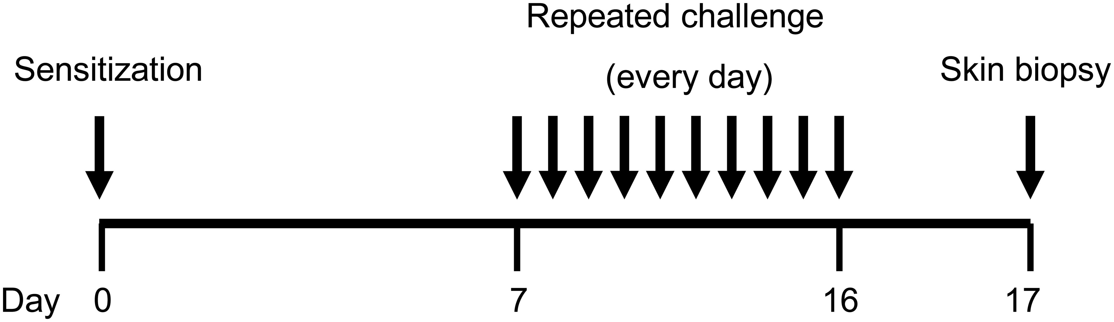
Kitagaki H, Fujisawa S, Watanabe K, et al. (1995) Immediate-type hypersensitivity response followed by a late reaction is induced by repeated epicutaneous application of contact sensitizing agents in mice. J Invest Dermatol 105: 749–755. doi: 10.1111/1523-1747.ep12325538
![]() |
[3] | Yamaura K, Shimada M, Ueno K (2011) Anthocyanins from bilberry (Vaccinium myrtillus L.) alleviate pruritus in a mouse model of chronic allergic contact dermatitis. Pharmacognosy Res 3: 173–177. |
[4] |
Boothe WD, Tarbox JA, Tarbox MB (2017) Atopic dermatitis: Pathophysiology. Adv Exp Med Biol 1027: 21–37. doi: 10.1007/978-3-319-64804-0_3
![]() |
[5] |
Lin L, Xie M, Chen X, et al. (2018) Toll-like receptor 4 attenuates a murine model of atopic dermatitis through inhibition of langerin-positive DCs migration. Exp Dermatol 27: 1015–1022. doi: 10.1111/exd.13698
![]() |
[6] |
Liu L, Guo D, Liang Q, et al. (2015) The efficacy of sublingual immunotherapy with Dermatophagoides farinae vaccine in a murine atopic dermatitis model. Clin Exp Allergy 45: 815–822. doi: 10.1111/cea.12417
![]() |
[7] |
Stander S, Steinhoff M (2002) Pathophysiology of pruritus in atopic dermatitis: An overview. Exp Dermatol 11: 12–24. doi: 10.1034/j.1600-0625.2002.110102.x
![]() |
[8] |
Seike M, Takata T, Ikeda M, et al. (2005) Histamine helps development of eczematous lesions in experimental contact dermatitis in mice. Arch Dermatol Res 297: 68–74. doi: 10.1007/s00403-005-0569-5
![]() |
[9] |
Seike M, Furuya K, Omura M, et al. (2010) Histamine H4 receptor antagonist ameliorates chronic allergic contact dermatitis induced by repeated challenge. Allergy 65: 319–326. doi: 10.1111/j.1398-9995.2009.02240.x
![]() |
[10] |
Matsushita A, Seike M, Okawa H, et al. (2012) Advantage of histamine H4 receptor antagonist usage with H1 receptor antagonist for the treatment of murine allergic contact dermatitis. Exp Dermatol 21: 714–715. doi: 10.1111/j.1600-0625.2012.01559.x
![]() |
[11] |
Ohsawa Y, Hirasawa N (2012) The antagonism of histamine H1 and H4 receptors ameliorates chronic allergic dermatitis via anti-pruritic and anti-inflammatory effects in NC/Nga mice. Allergy 67: 1014–1022. doi: 10.1111/j.1398-9995.2012.02854.x
![]() |
[12] |
Liang SC, Tan X, Luxenberg DP, et al. (2006) Interleukin (IL)-22 and IL-17 are coexpressed by Th17 cells and cooperatively enhance expression of antimicrobial peptides. J Exp Med 203: 2271–2279. doi: 10.1084/jem.20061308
![]() |
[13] |
Yi T, Chen Y, Wang L, et al. (2009) Reciprocal differentiation and tissue-specific pathogenesis of Th1, Th2 and Th17 cells in graft-versus-host disease. Blood 114: 3101–3112. doi: 10.1182/blood-2009-05-219402
![]() |
[14] |
Koga C, Kabashima K, Shiraishi N, et al. (2008) Possible pathogenic role of Th17 cells for atopic dermatitis. J Invest Dermatol 128: 2625–2630. doi: 10.1038/jid.2008.111
![]() |
[15] |
Matsushita A, Seike M, Hagiwara T, et al. (2014) Close relationship between T helper (Th)17 and Th2 response in murine allergic contact dermatitis. Clin Exp Dermatol 39: 924–931. doi: 10.1111/ced.12425
![]() |
[16] |
Ohtsu H, Tanaka S, Terui T, et al. (2001) Mice lacking histidine decarboxylase exhibit abnormal mast cells. FEBS Lett 502: 53–56. doi: 10.1016/S0014-5793(01)02663-1
![]() |
[17] |
Tamura T, Matsubara M, Takada C (2004) Effects of olopatadine hydrochloride, antihistamine drug, on skin inflammation induced by repeated topical application of oxazolone in mice. Brit J Dermatol 151: 1133–1142. doi: 10.1111/j.1365-2133.2004.06172.x
![]() |
[18] |
Kim JY, Jeong MS, Park MK, et al. (2014) Time-dependent progression from the acute to chronic phases in atopic dermatitis induced by epicutaneous allergen stimulation in NC/Nga mice. Exp Dermatol 23: 53–57. doi: 10.1111/exd.12297
![]() |
[19] |
Ohtsu H, Kuramasu K, Tanaka S, et al. (2002) Plasma extravasation induced by dietary supplemented histamine in histamine-free mice. Eur J Immunol 32: 1698–1708. doi: 10.1002/1521-4141(200206)32:6<1698::AID-IMMU1698>3.0.CO;2-7
![]() |
[20] |
Hamada R, Seike M, Kamijima R, et al. (2006) Neuronal conditions of spinal cord in dermatitis are improved by olopatadine. Eur J Pharmacol 547: 45–51. doi: 10.1016/j.ejphar.2006.06.058
![]() |
[21] |
Tamaka K, Seike M, Hagiwara T, et al. (2015) Histamine suppresses regulatory T cells mediated by TGF-β in murine chronic contact dermatitis. Exp Dermatol 24: 280–284. doi: 10.1111/exd.12644
![]() |
[22] |
Nakae S, Komiyama Y, Nambu A, et al. (2002) Antigen-specific T cell sensitization is impaired in IL-17-deficient mice, causing suppression of allergic cellular and humoral responses. Immunity 17: 375–387. doi: 10.1016/S1074-7613(02)00391-6
![]() |
[23] |
Zhao Y, Balato A, Fishelevich R, et al. (2009) Th17/Tc17 infiltration and associated cytokine gene expression in elicitation phase of allergic contact dermatitis. Brit J Dermatol 161: 1301–1306. doi: 10.1111/j.1365-2133.2009.09400.x
![]() |
[24] | Kim D, McAlees JW, Bischoff LJ, et al. (2018) Combined administration of anti-IL-13 and anti-IL-17A at individually sub-therapeutic doses limits asthma-like symptoms in a mouse model of Th2/Th17 high asthma. Clin Exp Allergy, 24. |
[25] |
Bian R, Tang J, Hu L, et al. (2018) (E)-phenethyl 3-(3,5-dihydroxy-4-isopropylphenyl) acrylate gel improves DNFB-induced allergic contact hypersensitivity via regulating the balance of Th1/Th2/T17/Treg cell subsets. Int Immunopharmacol 65: 8–15. doi: 10.1016/j.intimp.2018.09.032
![]() |
[26] |
Wu R, Zeng J, Yuan J, et al. (2018) MicroRNA-210 overexpression promotes psoriasis-like inflammation by inducing Th1 and Th17 cell differentiation. J Clin Invest 128: 2551–2568. doi: 10.1172/JCI97426
![]() |
[27] |
Orciani M, Campanati A, Caffarini M, et al. (2017) T helper (Th)1, Th17 and Th2 imbalance in mesenchymal stem cells of adult patients with atopic dermatitis: at the origin of the problem. Brit J Dermatol 176: 1569–1576. doi: 10.1111/bjd.15078
![]() |
[28] |
Harrington LE, Hatton RD, Mangan PR, et al. (2005) Interleukin 17-producing CD4+ effector T cells develop via a lineage distinct from the T helper type 1 and 2 lineage. Nat Immunol 6: 1123–1132. doi: 10.1038/ni1254
![]() |
[29] |
Mangan PR, Harrington LE, O'Quinn DB, et al. (2006) Transforming growth factor-beta induces development of the TH17 lineage. Nature 441: 231–234. doi: 10.1038/nature04754
![]() |
1. | B. Amaziane, L. Pankratov, A. Piatnitski, Homogenization of immiscible compressible two–phase flow in random porous media, 2021, 305, 00220396, 206, 10.1016/j.jde.2021.10.012 | |
2. | Hadi Hajibeygi, Manuela Bastidas Olivares, Mousa HosseiniMehr, Sorin Pop, Mary Wheeler, A benchmark study of the multiscale and homogenization methods for fully implicit multiphase flow simulations, 2020, 143, 03091708, 103674, 10.1016/j.advwatres.2020.103674 | |
3. | B. Amaziane, L. Pankratov, Homogenization of coupled immiscible compressible two-phase flow with kinetics in porous media, 2022, 101, 0003-6811, 241, 10.1080/00036811.2020.1738398 | |
4. | B. Amaziane, M. Jurak, L. Pankratov, A. Piatnitski, Homogenization of nonisothermal immiscible incompressible two-phase flow in porous media, 2018, 43, 14681218, 192, 10.1016/j.nonrwa.2018.02.012 | |
5. | M. Jamei, A. Raeisi Isa Abadi, I. Ahmadianfar, A Lax–Wendroff-IMPES scheme for a two-phase flow in porous media using interior penalty discontinuous Galerkin method, 2019, 75, 1040-7790, 325, 10.1080/10407790.2019.1627825 | |
6. | B. Amaziane, M. Jurak, L. Pankratov, A. Piatnitski, Homogenization of nonisothermal immiscible incompressible two-phase flow in double porosity media, 2021, 61, 14681218, 103323, 10.1016/j.nonrwa.2021.103323 | |
7. | Brahim Amaziane, Mladen Jurak, Leonid Pankratov, Andrey Piatnitski, An existence result for nonisothermal immiscible incompressible 2-phase flow in heterogeneous porous media, 2017, 40, 01704214, 7510, 10.1002/mma.4544 |