Citation: Christian M. Julien, Alain Mauger. In situ Raman analyses of electrode materials for Li-ion batteries[J]. AIMS Materials Science, 2018, 5(4): 650-698. doi: 10.3934/matersci.2018.4.650
[1] | Vivek Tewary . Combined effects of homogenization and singular perturbations: A bloch wave approach. Networks and Heterogeneous Media, 2021, 16(3): 427-458. doi: 10.3934/nhm.2021012 |
[2] | Grégoire Allaire, Tuhin Ghosh, Muthusamy Vanninathan . Homogenization of stokes system using bloch waves. Networks and Heterogeneous Media, 2017, 12(4): 525-550. doi: 10.3934/nhm.2017022 |
[3] | Carlos Conca, Luis Friz, Jaime H. Ortega . Direct integral decomposition for periodic function spaces and application to Bloch waves. Networks and Heterogeneous Media, 2008, 3(3): 555-566. doi: 10.3934/nhm.2008.3.555 |
[4] | Laura Caravenna, Laura V. Spinolo . New interaction estimates for the Baiti-Jenssen system. Networks and Heterogeneous Media, 2016, 11(2): 263-280. doi: 10.3934/nhm.2016.11.263 |
[5] | Riccardo Bonetto, Hildeberto Jardón Kojakhmetov . Nonlinear diffusion on networks: Perturbations and consensus dynamics. Networks and Heterogeneous Media, 2024, 19(3): 1344-1380. doi: 10.3934/nhm.2024058 |
[6] | Rémi Goudey . A periodic homogenization problem with defects rare at infinity. Networks and Heterogeneous Media, 2022, 17(4): 547-592. doi: 10.3934/nhm.2022014 |
[7] | Andrea Braides, Valeria Chiadò Piat . Non convex homogenization problems for singular structures. Networks and Heterogeneous Media, 2008, 3(3): 489-508. doi: 10.3934/nhm.2008.3.489 |
[8] | Hiroshi Matano, Ken-Ichi Nakamura, Bendong Lou . Periodic traveling waves in a two-dimensional cylinder with saw-toothed boundary and their homogenization limit. Networks and Heterogeneous Media, 2006, 1(4): 537-568. doi: 10.3934/nhm.2006.1.537 |
[9] | Hakima Bessaih, Yalchin Efendiev, Florin Maris . Homogenization of the evolution Stokes equation in a perforated domain with a stochastic Fourier boundary condition. Networks and Heterogeneous Media, 2015, 10(2): 343-367. doi: 10.3934/nhm.2015.10.343 |
[10] | Antonin Chambolle, Gilles Thouroude . Homogenization of interfacial energies and construction of plane-like minimizers in periodic media through a cell problem. Networks and Heterogeneous Media, 2009, 4(1): 127-152. doi: 10.3934/nhm.2009.4.127 |
The formation of shear bands in elasticity is described by a degenerate operator of elliptic-hyperbolic type [1, 23, 4]. The shear bands that are mathematically obtained in this model are infinitesimally thin. To overcome this non-physical description, it is customary to penalize the elasticity operator by a fourth-order singular perturbation [18]. Subsequently, it was suggested that the penalization should be followed by a homogenization procedure, which results in different regimes depending on the order of penalization as compared to the length-scale of the periodic heterogeneities. This was first carried out in [6, 18]. Similar problems in the framework of
We will study the simultaneous homogenization and singular perturbation limits of the following operator
Aκ,ε:=κ2Δ2−∇⋅A(xε)∇, | (1.1) |
where
A1.
A2.
A3. The matrix
We mention briefly the function spaces that make an appearance in this problem. The solutions of the cell problem associated with homogenization of (1.1), as well as Bloch eigenfunctions, are sought in the space .
The method of Bloch waves rests on decomposition of a periodic operator in terms of Bloch waves which may be thought of as a periodic analogue of plane waves. As plane waves decompose a linear operator with constant coefficients by means of the Fourier transform, Bloch waves diagonalize a linear operator with periodic coefficients. This decomposition begins with a direct integral decomposition of a periodic operator
A→⨁∫TdA(η)dη. |
The fiber operator
The homogenization limits for a highly oscillating scalar periodic operator are obtained from its first Bloch mode. The rest of the Bloch modes do not contribute to the homogenization limit. This is a consequence of the separation of the first Bloch eigenvalue from the rest of the spectrum. Such an interpretation of homogenization is also called spectral threshold effect [7]. Moreover, the homogenized tensor is obtained from Hessian of the first Bloch eigenvalue. Therefore, the second-order nature of the differential operator is reflected in the quadratic nature of the first Bloch eigenvalue near the bottom of the spectrum. Indeed, homogenization of higher-even-order periodic operators can also be obtained by the Bloch wave method, where the first Bloch eigenvalue behaves like a polynomial of the corresponding order near the bottom of the spectrum [37, 36].
The homogenization result in Theorem 8.1 exhibits three different regimes depending on the ratio of
●
●
●
In the first regime, the subcritical case, that is,
The approach is to treat
While the motivation for the problem (1.1) comes from the theory of elasticity, it is for the sake of simplicity that we only study the scalar operator. However, it must be noted that Bloch wave homogenization of systems carries some unique difficulties, such as the presence of multiplicity at the bottom of the spectrum. Indeed, these challenges have been surmounted by the use of directional analyticity of Bloch eigenvalues in [35, 7, 3]. Further, the assumption of symmetry, while customary in elasticity, is made for a simplified presentation. A Bloch wave analysis of homogenization of non-selfadjoint operators may be found in [19].
In a forthcoming work, we will obtain quantitative estimates for the combined effects of singular perturbation and homogenization through the notion of Bloch approximation, which was introduced in [11]. Higher order estimates in homogenization have been obtained by these methods, particularly for the dispersive wave equation [14, 15, 2, 22].
The plan of the paper is as follows: In Section 2, we obtain Bloch waves for the singularly perturbed operator
In this section, we will prove the existence of Bloch waves for the singular operator given by
Aρ:=ρ2Δ2−∇⋅A(y)∇. | (2.1) |
Recall that
{ρ2Δ2ψ−∇⋅A(y)∇ψ=λψψ(y+2πp)=e2πip⋅ηψ(y),p∈Zd,η∈Rd. |
The above problem is invariant under
{Aρ(η)ϕ:=ρ2(∇+iη)4ϕ−(∇+iη)⋅A(y)(∇+iη)ϕ=λϕϕ(y+2πp)=ϕ(y),p∈Zd,η∈Y′. | (2.2) |
The operator
The bilinear form
aρ[η](u,v):=∫YA(∇+iη)u⋅¯(∇+iη)vdy+ρ2∫Y(∇+iη)2u¯(∇+iη)2vdy, | (2.3) |
is associated to the operator
Lemma 2.1. There exists a positive real number
aρ[η](u,u)+C∗||u||2L2♯(Y)≥ρ26||Δu||2L2♯(Y)+α2||u||H1♯(Q). | (2.4) |
Proof. We have
aρ[η](u,u)=∫YA(∇+iη)u⋅¯(∇+iη)udy⏟I+ρ2∫Y(∇+iη)2u¯(∇+iη)2udy⏟II. | (2.5) |
We shall estimate the two summands separately. For the first summand, observe that
I=∫YA(∇+iη)u⋅¯(∇+iη)udy=∫YA∇u⋅¯∇udy+2Re{∫YAiηu⋅¯∇udy}+∫YAηu⋅η¯udy, | (2.6) |
where
∫YA∇u⋅∇¯udy=∫YA∇u⋅∇¯udy≥α∫Y|∇u|2dy. | (2.7) |
For the second term of
|2Re{∫YAηu⋅∇¯udy}|≤2∫Y|Aηu⋅∇¯u|dy≤C1∫Y|ηu⋅∇¯u|dy≤C1||ηu||L2♯(Y)||∇u||L2♯(Y)≤C1C2||u||2L2♯(Y)+C1C2||∇u||L2♯(Y). | (2.8) |
Finally, the third term of
|∫YAηu⋅η¯udy|≤C3∫Y|ηu⋅η¯u|dy≤C4||u||L2♯(Y). | (2.9) |
Now, we may choose
I≥α2||u||L2♯(Y)+α2||∇u||L2♯(Y)−(α2+C1C2+C4)||u||2L2♯(Y). | (2.10) |
For the second summand, observe that
II=ρ2∫Y|(∇+iη)2u|2dy=ρ2∫Y|Δu|2dy+ρ2∫Y|η|4|u|2dy+4ρ2∫Y|η⋅∇u|2dy+2ρ2iIm{∫Y|η|2u¯Δudy}+4iρ2Re{∫Y(η⋅∇u)Δ¯udy}+4iρ2Re{∫Y|η|2u(η⋅∇¯u)dy}. | (2.11) |
We estimate the last three terms as follows.
ρ2|2iIm{∫Y|η|2u¯Δudy}|≤2ρ2∫Y|η|2|u||Δu|dy≤2ρ2|η|2||u||L2||Δu||L2≤48ρ2|η|4||u||2L2+ρ248||Δu||2L2. | (2.12) |
ρ2|4iRe{∫Y(η⋅∇)uΔ¯udy}|≤4ρ2∫Y|(η⋅∇)u||Δu|dy≤4ρ2||(η⋅∇)u||L2||Δu||L2≤16ρ23||(η⋅∇)u||2L2+3ρ24||Δu||2L2. | (2.13) |
ρ2|4iRe{∫Y|η|2u(η⋅∇)¯udy}|≤4ρ2∫Y|(η⋅∇)u||η|2|u|dy≤4ρ2|η|2||u||L2||(η⋅∇)u||L2≤192ρ2|η|4||u||2L2+ρ248||(η⋅∇)u||2L2. | (2.14) |
The previous threee estimate use Cauchy-Schwarz inequality for the second step and Young's inequality for the third step. Substituting the inequalities (2.12), (2.13) and (2.14) into (2.11), we get
II≥11ρ248||Δu||2L2(Y)−240ρ2|η|4||u||2L2(Y)−65ρ248||(η⋅∇)u||2L2(Y). | (2.15) |
Since
II≥11ρ248||Δu||2L2(Y)−15ρ2||u||2L2(Y)−65ρ2192||∇u||2L2(Y). |
Now, notice that
||∇u||2L2=∫Y|∇u|2dy=−∫YuΔudy≤6548||u||2L2+1265||Δu||2L2. | (2.16) |
Substituting (2.16) in (2.15), we get
II≥ρ26||Δu||2L2(Y)−16ρ2||u||2L2(Y). | (2.17) |
Combining (2.10) and (2.17), we obtain (2.4) with
C∗=(α2+C1C2+C4+16ρ2). | (2.18) |
Remark 2.2. In the Gå rding type inequality for the operator
Now that we have the coercivity estimate (2.4), we can prove the existence of Bloch eigenvalues and eigenfunctions for the operator
Theorem 2.3. For each
Proof. Lemma 2.1 shows that for every
Remark 2.4. We can prove the existence of Bloch eigenvalues and eigenfunctions for the case
Now that we have proved the existence of Bloch eigenvalues and eigenfunctions, we can state the Bloch Decomposition Theorem which offers a partial diagonalization of the operator
Theorem 2.5. Let
Bρmg(η):=∫Rdg(y)e−iy⋅η¯ϕρm(y;η)dy,m∈N,η∈Y′. | (2.19) |
1. The following inverse formula holds
g(y)=∫Y′∞∑m=1Bρmg(η)ϕρm(y;η)eiy⋅ηdη. | (2.20) |
2. Parseval's identity
||g||2L2(Rd)=∞∑m=1∫Y′|Bρmg(η)|2dη. | (2.21) |
3. Plancherel formula For
∫Rdf(y)¯g(y)dy=∞∑m=1∫Y′Bρmf(η)¯Bρmg(η)dη. | (2.22) |
4. Bloch Decomposition in
BρmF(η)=∫Rde−iy⋅η{u0(y)¯ϕρm(y;η)+iN∑j=1ηjuj(y)¯ϕρm(y;η)}dy−∫Rde−iy⋅ηN∑j=1uj(y)∂¯ϕρm∂yj(y;η)dy. | (2.23) |
The definition above is independent of the particular representative of
5. Finally, for
Bρm(Aρg)(η)=λρm(η)Bρmg(η). | (2.24) |
The Bloch wave method of homogenization requires differentiability of the Bloch eigenvalues and eigenfunctions in a neighbourhood of
Theorem 3.1. For every
1. The first Bloch eigenvalue
2. There is a choice of corresponding eigenfunctions
For the proof, we will make use of Kato-Rellich theorem which establishes the existence of a sequence of eigenvalues and eigenfunctions associated with a selfadjoint holomorphic family of type (B). The definition of selfadjoint holomorphic family of type (B) and other related notions may be found in Kato [21]. Nevertheless, they are stated below for completeness. We begin with the definition of a holomorphic family of forms of type (a).
Definition 3.2.
1. The numerical range of a form
Θ(a)={a(u,u):u∈D(a),||u||=1} |
where
2. The form
Θ(a)⊂Sc,θ:={λ∈C:|arg(λ−c)|≤θ)}. |
3. A sectorial form
Definition 3.3. [Kato] A family of forms
1. each
2.
A family of operators is called a holomorphic family of type (B) if it generates a holomorphic family of forms of type (a).
In [21, 31], Kato-Rellich theorem is stated only for a single parameter family. In [5], one can find the proof of Kato-Rellich theorem for multiple parameters with the added assumption of simplicity for the eigenvalue at
Theorem 3.4. (Kato-Rellich) Let
1. There is exactly one point
2. There is an associated eigenfunction
The proof of Theorem 3.1 proceeds by complexifying the shifted operator
Proof. (Proof of Theorem 3.1)
(i) Complexification of
t(˜η)=∫YA(∇+iσ−τ)u⋅(∇−iσ+τ)¯udy+ρ2∫Y|(∇+iσ+τ)2u|2dy |
for
R:={˜η∈CM:˜η=σ+iτ,σ,τ∈RM,|σ|<1/2,|τ|<1/2}. |
(ii) the form
t(˜η)=∫YA(∇+iσ−τ)u⋅(∇−iσ+τ)¯udy+ρ2∫Y|(∇+iσ+τ)2u|2dy=∫YA(∇+iσ)u⋅(∇−iσ)¯udy−∫YA(τu)⋅∇¯udy+∫YA∇u⋅(τ¯u)dy−∫YAτu⋅τ¯udy+i∫YAσu⋅τ¯udy+i∫YAτu⋅σ¯udy+ρ2∫Y(Δ−|σ|2+|τ|2)u(Δ−|σ|2+|τ|2)¯udy+2ρ2∫Y(Δ−|σ|2+|τ|2)u(τ⋅∇−iσ⋅∇−iσ⋅τ)¯udy+2ρ2∫Y(iσ⋅∇−τ⋅∇−iσ⋅τ)u(Δ−|σ|2+|τ|2)¯udy+4ρ2∫Y(iσ⋅∇−τ⋅∇−iσ⋅τ)u(τ⋅∇−iσ⋅∇−iσ⋅τ)¯udy. |
From above, it is easy to write separately the real and imaginary parts of the form
ℜt(˜η)[u]=∫YA(∇+iσ)u⋅(∇−iσ)¯udy−∫YAτu⋅τ¯udy+ρ2∫Y(Δ−|σ|2+|τ|2)u(Δ−|σ|2+|τ|2)¯udy−4ρ2∫Y|(τ⋅∇)u|2dy+4ρ2∫Y|(σ⋅∇)u|2dy−4ρ2∫Y|(τ⋅σ)u|2dy+8ρ2Re{∫Yi(τ⋅∇)u(σ⋅τ)¯udy}+4ρ2Re{∫Yi(σ⋅∇)uΔ¯udy}+4ρ2Re{∫Yi|σ|2u(σ⋅∇)¯udy}. |
ℑt(˜η)[u]=∫YAσu⋅τ¯udy+∫YAτu⋅σ¯udy+2ℑ{∫YA∇u⋅τ¯udy}+8ρ2Im{∫Yi(τ⋅σ)u(σ⋅∇)¯udy}+8ρ2Im{∫Yi(σ⋅∇)u(σ⋅τ)¯udy}+4ρ2Im{∫YΔu(τ⋅∇)¯udy}−4ρ2Im{∫YiΔu(σ⋅τ)¯udy}+4ρ2Im{∫Y(τ⋅∇)u|σ|2¯udy}+4ρ2Im{∫Yi|σ|2u(σ⋅τ)¯udy}+4ρ2Im{∫Y|τ|2u(τ⋅∇)¯udy}−4ρ2Im{∫Yi|τ|2u(σ⋅τ)¯udy}. |
The following coercivity estimate can be easily found for the real part:
ℜt(˜η)[u]+C5||u||2L2♯(Y)≥α2(||u||2L2♯(Y)+||∇u||2L2♯(Y))+ρ26||Δu||2L2♯(Y). | (3.1) |
Let us define the new form
ℜ˜t(˜η)[u]≥α2(||u||2L2♯(Y)+||∇u||2L2♯(Y))+ρ26||Δu||2L2♯(Y)+C6||u||2L2♯(Y). |
Also, the imaginary part of
ℑ˜t(˜η)[u]≤C7||u||2L2♯(Y)+C8||∇u||2L2♯(Y)+C9||Δu||2L2♯(Y)C10=max{2C8α,6C9ρ2}=C6=C10C7C10(C6||u||2L2♯(Y)+α2||∇u||2L2♯(Y)+ρ26||Δu||2L2♯(Y))≤C10(ℜ˜t(˜η)[u]−α2||u||2L2♯(Y)). |
This shows that
(iii) The form
(iv) The form
(v)
(vi)
(vii)
In Section 3, we have proved that the first Bloch eigenvalue and eigenfunction is analytic in a neighbourhood of
We begin by proving that Bloch eigenvalues are Lipschitz continuous in the dual parameter.
Lemma 4.1. For all
Proof. The following form is associated with
aρ[η](u,u)=∫YA(∇+iη)u⋅¯(∇+iη)udy+ρ2∫Y(∇+iη)2u¯(∇+iη)2udy. | (4.1) |
Hence, for
aρ[η]−aρ[η′]=2Re{∫YAi(η−η′)u⋅¯∇udy}+∫YAηu⋅η¯udy+∫YAη′u⋅η′¯udy+ρ2∫Y(|η|2−|η′|2)|u|2dy+4ρ2∫Y|η⋅∇u|2−|η′⋅∇u|2dy+2ρ2iIm{∫Y(|η|2−|η′|2)uΔ¯udy}+4ρ2iRe{∫Y(η−η′)⋅∇uΔ¯udy}+4ρ2iRe{∫Y|η|2u(η⋅∇)¯u−|η′|2u(η′⋅∇)¯udy}≤C|η−η′|||u||2H1♯(Y)+C′|η−η′|ρ2{||Δu||2L2♯(Y)+||u||2L2♯(Y)}, |
where
λρm(η)≤λρm(η′)+C|η−η′|μm+C′ρ2|η−η′|νm, | (4.2) |
where
{−Δum+um=μmuminYumisY−periodic, |
and
{Δ2vm+vm=νmvminYvmisY−periodic. |
By interchanging the role of
|λρm(η)−λρm(η′)|≤C(μm+ρ2νm)|η−η′|. | (4.3) |
Here,
Now, we will prove a spectral gap result, viz. the second Bloch eigenvalue is bounded below.
Lemma 4.2. For all
λρm(η)≥αλN2, | (4.4) |
where
Proof. Notice that
λρ2(η)=infW⊂H2♯(Y)dim(W)=2maxϕ∈Wϕ≠0∫YA∇(eiη⋅yϕ)⋅∇(e−iη⋅y¯ϕ)dy+ρ2∫Y|Δ(eiη⋅yϕ)|2dy∫Y|ϕ|2dy≥infW⊂H2(Y)dim(W)=2maxψ∈Wψ≠0∫YA∇ψ⋅∇¯ψdy+ρ2∫Y|Δψ|2dy∫Y|ψ|2dy≥infW⊂H2(Y)dim(W)=2maxψ∈Wψ≠0∫YA∇ψ⋅∇¯ψdy∫Y|ψ|2dy≥infW⊂H1(Y)dim(W)=2maxψ∈Wψ≠0∫YA∇ψ⋅∇¯ψdy∫Y|ψ|2dy≥αinfW⊂H1(Y)dim(W)=2maxψ∈Wψ≠0∫Y|∇ψ|2dy∫Y|ψ|2dy=αλN2. |
The bound obtained in Lemma 4.2 will be useful for the small
Lemma 4.3. For all
λρm(η)≥Cρ2κ2−C′, | (4.5) |
where
Proof. Recall the following Gå rding type estimate (2.4) for the form
aρ[η](u,u)+C∗||u||2L2♯(Y)≥ρ26||Δu||2L2♯(Y)+α2||u||H1♯(Q). |
The inequality in Lemma 4.3 follows readily from above by applying the minmax characterization.
Remark 4.4. In Lemma 4.2 and Lemma 4.3, we have avoided estimating the second Bloch eigenvalue by using the spectral problem associated with Neumann bilaplacian as it is known to be ill-posed [30]. Moreover, polyharmonic Neumann eigenvalue problems on polygonal domains (such as
We are finally in a position to prove that the neighbourhood of analyticity of the first Bloch eigenvalue does not depend on the parameter
Theorem 4.5. There exists a neighbourhood
Proof. It was proved in Theorem 3.1 that the first Bloch eigenvalue is analytic in a neighbourhood of
|λρ1(η)−λρ2(η)|≥λρ2(η)−|λρ1(η)−λρ1(0)|−|λρ2(η)−λρ2(0)|(4.3)≥λρ2(η)−2(C+ρ2)|η|, | (4.6) |
where
● For sufficiently large
|λρ1(η)−λρ2(η)|≥λρ2(η)−2(C+ρ2)|η|Lemma4.3≥(C′ρ2−C″)−2(C+ρ2)|η|largeρ≥C‴ρ2−2ρ2|η|>0 |
for
● For remaining values of
|λρ1(η)−λρ2(η)|≥λρ2(η)−2(C+ρ2)|η|Lemma4.2≥αλN2−2(C+ρ2)|η|≥αλN2−2C|η|>0 |
for
Remark 4.6. In the papers [33, 34], an additional artificial parameter is introduced in the Bloch eigenvalue problem to facilitate the homogenization method. Unlike (1.1), these papers employ successive limits of the two parameters instead of simultaneous limits. Therefore, the non-dependence of the neighbourhood of analyticity on the second parameter is not required in [33, 34].
In this section, we will consider the classical cell problem associated with (1.1) and the estimates for the corrector field. This section will allow us to characterize the homogenized tensor for (1.1) and the corrector field in terms of Bloch eigenvalues and eigenfunctions.
For
(5.1) |
By a simple application of Lax-Milgram lemma on
ρ||Δχρj||L2♯(Y)+||χρj||H1♯(Y)≤C. | (5.2) |
If we use
ρ2||∇3χρj||L2♯(Y)≤C. | (5.3) |
We also collect below a few estimates which will be required later. Similar estimates have been proved in [26] to which we refer for more details.
Lemma 5.1. Let
||∇χρ1−∇χρ2||L2(Y)≤C|1−(ρ1/ρ2)2|. | (5.4) |
Proof. Define
ρ21Δ2z−divA(y)∇z=(ρ22−ρ21)Δ2χρ2. | (5.5) |
Now, the quoted estimate readily follows by taking
Lemma 5.2. Let
(5.6) |
Then, there is
||∇χ0j−∇χBj||L2(Y)≤Cϰ | (5.7) |
||∇χρ−∇χB||L2(Y)≤C{ρ||χB||H2(Y)+ϰ}, | (5.8) |
where
(5.9) |
Proof. Observe that given any
||A−B||Lq♯(Y)≤ϰ. |
For example, this can be achieved by a standard smoothing by convolution. Now, by regularity theory,
ρ2Δ2z−divB(y)∇z=−ρ2Δ2χBj+div(A−B)∇χρj. | (5.10) |
We test this equation against
ρ2∫Y|Δz|2dy+∫YA(y)∇z⋅∇zdy≤ρ2∫Y|ΔχBj||Δz|dy+∫Y|A−B||∇χρj||∇z|dy. |
This leads to
ρ2||Δz||2L2+α||∇z||2L2≤ρ2||ΔχBj||L2||Δz||L2+||∇z||L2(∫Y|A−B|2|∇χρj|2dy)1/2. |
By Young's inequality,
||∇z||L2≤C{ρ||ΔχBj||L2+(∫Y|A−B|2|∇χρj|2dy)1/2}. |
On the last term, we apply a form of Meyers estimate for the
For every fixed
Aρ,hom:=MY(A+A∇χρ) | (5.11) |
Definition 5.3 (Homogenized Tensor for
Ahom:={MY(A+A∇χθ)for0<θ<∞whereρ=κε→θ,MY(A+A∇χ0)whenρ=κε→0,MY(A)whenρ=κε→∞. | (5.12) |
In this section, we will give a new characterization of the homogenized tensor (see Definition 5.3), and corrector field (5.1) in terms of the first Bloch eigenvalue and eigenfunction. These characterizations are obtained by differentiating the Bloch spectral problem (2.2) with respect to the dual parameter
We recall the Bloch eigenvalue problem for the operator
ρ2(∇+iη)4ϕρ1(y;η)−(∇+iη)⋅A(y)(∇+iη)ϕρ1(y;η)=λρ1(η)ϕρ1(y;η). | (6.1) |
We know that
We shall normalize the average value of the first Bloch eigenfunction
MY(ϕρ1(⋅,η))=(2π)−d/2 | (6.2) |
for all
MY(∂β0ϕρ1)=0 | (6.3) |
for all
∂βηA≡0forall|β|>4, | (6.4) |
since
Aρ(0)=ρ2∇4−∇⋅A(y)∇∂ej0Aρ=4iρ2ej⋅∇∇2−iej⋅A∇−i∇⋅Aej∂ej+ek0Aρ=−4ρ2δjk∇2−8ρ2∂yj∂yk+2ajk∂ej+ek+el0Aρ=−8iρ2(δjk∂yl+δjl∂yk+δkl∂yj)∂ej+ek+el+em0Aρ=8ρ2(δjkδlm+δjlδkm+δjmδkl), | (6.5) |
where
∂β(fg)=∑γ∈Nd∪{0}(βγ)∂γf∂β−γg, | (6.6) |
where
Cell problems for
Aρ(0)∂β0ϕρ1+d∑j=1βj∂ej0Aρ∂β−ej0ϕρ1+∑j,k(βej+ek)∂ej+ek0Aρ∂β−ej−ek0ϕρ1 |
+∑j,k,l(βej+ek+el)∂ej+ek+el0Aρ∂β−ej−ek−el0ϕρ1+∑j,k,l,m(βej+ek+el+em)∂ej+ek+el+em0Aρ∂β−ej−ek−el−em0ϕρ1=∑γ∈Nd∪{0}(βγ)∂γ0λρ1∂β−γ0ϕρ1. | (6.7) |
Substituting (6.5) in (6.7), we obtain
(ρ2∇4−∇⋅A(y)∇)∂β0ϕρ1=d∑j=1βj(−4iρ2ej⋅∇∇2+iej⋅A∇+i∇⋅Aej)∂β−ej0ϕρ1−∑j,k(βej+ek)(−4ρ2δjk∇2−8ρ2∂yj∂yk+2ajk)∂β−ej−ek0ϕρ1+∑j,k,l(βej+ek+el)(8iρ2(δjk∂yl+δjl∂yk+δkl∂yj))∂β−ej−ek−el0ϕρ1−∑j,k,l,m(βej+ek+el+em)(8ρ2(δjkδlm+δjlδkm+δjmδkl))∂β−ej−ek−el−em0ϕρ1+∑γ∈Nd(βγ)∂γ0λρ1∂β−γ0ϕρ1. | (6.8) |
Expression for
Rearranging (6.8), we get
∂β0λρ1ϕρ1(0)=(ρ2∇4−∇⋅A(y)∇)∂β0ϕρ1+d∑j=1βj(−4iρ2ej⋅∇∇2+iej⋅A∇+i∇⋅Aej)∂β−ej0ϕρ1−∑j,k(βej+ek)(−4ρ2δjk∇2−8ρ2∂yj∂yk+2ajk)∂β−ej−ek0ϕρ1+∑j,k,l(βej+ek+el)(8iρ2(δjk∂yl+δjl∂yk+δkl∂yj))∂β−ej−ek−el0ϕρ1−∑j,k,l,m(βej+ek+el+em)(8ρ2(δjkδlm+δjlδkm+δjmδkl))∂β−ej−ek−el−em0ϕρ1+∑γ∈Ndγ≠β(βγ)∂γ0λρ1∂β−γ0ϕρ1. | (6.9) |
Integrating (6.9) over
∂β0λρ1={2∑j,k(βej+ek)MY(ajk∂β−ej−ek0ϕρ1)−id∑j=1βjMY(ej⋅A∇∂β−ej0ϕρ1)when|β|≠4.2∑j,k(βej+ek)MY(ajk∂β−ej−ek0ϕρ1)−id∑j=1βjMY(ej⋅A∇∂β−ej0ϕρ1)−∑j,k,l,m8ρ2(δjkδlm+δjlδkm+δjmδkl)ϕρ1(0)when|β|=4. | (6.10) |
We specialize to
On the other hand, if we set
(−∇⋅A(y)∇+ρ2Δ2)∂ϕρ1∂ηl(0)=∇⋅A(y)eliϕρ1(0). |
Comparing with (5.1), we conclude that
We also specialize to
12∂2λρ1∂ηk∂ηl(0)=1|Y|∫Y(ek⋅Ael+12ek⋅A∇χρl+12el⋅A∇χρk)dy. | (6.11) |
On comparing (6.11) with (5.11), we obtain the following theorem:
Theorem 6.1. The first Bloch eigenvalue and eigenfunction satisfy:
1.
2. The eigenvalue
∂λρ1∂ηl(0)=0,∀l=1,2,…,d. | (6.12) |
3. For
4. The Hessian of the first Bloch eigenvalue at
12∂2λρ1∂ηk∂ηl(0)=ek⋅Aρ,homel. | (6.13) |
Now, we will prove the stability of homogenized tensor in the limits
Lemma 6.2. Let
Proof. The fact that the first Bloch eigenvalues
|λρ1(η)|≤|λρ1(η)−λρ1(0|(4.3)≤C(μ1+ν1ρ2)|η|<C′forallη∈K, |
where
aρ[η](u,u)=∫YA(∇+iη)u⋅¯(∇+iη)udy+ρ2∫Y(∇+iη)2u¯(∇+iη)2udy=aθ[η](u,u)+(ρ2−θ2)∫Y(∇+iη)2u¯(∇+iη)2udy |
we obtain the following inequality:
λρ1(η)−λθ1(η)≤(ρ2−θ2)ϑ1(η), |
where
aρ[η](u,u)≥aθ[η](u,u)forρ≥θ, |
so that an application of minmax characterization yields:
λρ1(η)≥λθ1(η)forρ≥θ. |
Thus, we obtain
0≤λρ1(η)−λθ1(η)≤(ρ2−θ2)ϑ1(η)forρ≥θ. |
As a consequence, for each
Theorem 6.3. Let
Proof.
Case 1.
Aρ,hom=12∇2ηλρ1(0)→12∇2ηλθ1(0)=Ahomasρ↓θ∈[0,∞). |
Case 2.
|Aρ,hom−MY(A)|=|∫YA(y)∇χρ(y)dy|≤C||∇χρ||L2♯(Y)≤Cρ2, |
where the last inequality follows from Poincaré inequality and (5.3). Therefore, as
Aρ,hom→MY(A)=Ahomasρ↑∞. |
Remark 6.4. As a consequence of Lemma 6.2 and the discussion in Case
|λρ1(η)|+C∗≥λρ1(η)+C∗=aρ[η](ϕρ1(η),ϕρ1(η))+C∗≥α2||ϕρ1(η)||2H1♯(Y). |
Recall that the number
We end this section by finding boundedness estimates for higher order derivatives of the first Bloch eigenvalue and eigenfunction in the dual parameter in the regime
Theorem 6.5. For
1.
2.
3.
4.
5.
Proof. The estimates are computed in tandem from the equations (6.8) and (6.10). One begins by proving the estimate on the derivative of the first Bloch eigenfunction at
In this section, we will relate the Bloch spectral problem (2.2) to the Bloch spectral problem at the
\begin{eqnarray} \begin{cases} \mathcal{A}^{\kappa, \varepsilon}(\eta)\phi^{\kappa, \varepsilon}&:= \kappa^2(\nabla+i\xi)^4\phi^{\kappa, \varepsilon}(x)-(\nabla+i\xi)\cdot A\left(\frac{x}{ \varepsilon}\right)(\nabla+i\xi)\phi^{\kappa, \varepsilon}(x)\\ &\qquad = \lambda^{\kappa, \varepsilon}(\xi)\phi^{\kappa, \varepsilon}(x)\\ \phi^{\kappa, \varepsilon}(x+2\pi p \varepsilon)& = \phi^{\kappa, \varepsilon}(x), p\in\mathbb{Z}^d,\xi\in \frac{Y^{'}}{ \varepsilon}. \end{cases} \end{eqnarray} | (7.1) |
Comparing to (2.2), by homothety and
\begin{align} \lambda^{\kappa, \varepsilon}(\xi) = \varepsilon^{-2}\lambda^\rho( \varepsilon\xi){\rm{ and }}\phi^{\kappa, \varepsilon}(x,\xi) = \phi^\rho\left(\frac{x}{ \varepsilon}; \varepsilon\xi\right). \end{align} | (7.2) |
Now, we can state the Bloch decomposition theorem of
Theorem 7.1. Let
\begin{align} \mathcal{B}^{\kappa, \varepsilon}_mg(\xi):=\int_{\mathbb{R}^d}g(x)e^{-ix\cdot\xi}\overline{\phi_m^{\kappa, \varepsilon}(x;\xi)}\,dx,\; m\in\mathbb{N},\; \xi\in \frac{Y^{'}}{ \varepsilon}. \end{align} | (7.3) |
1. The following inverse formula holds
\begin{align} g(x) = \int_{\frac{Y^{'}}{ \varepsilon}}\sum\limits_{m = 1}^{\infty}\mathcal{B}^{\kappa, \varepsilon}_mg(\xi)\phi_m^{\kappa, \varepsilon}(x;\xi)e^{ix\cdot\xi}\,d\xi. \end{align} | (7.4) |
2. Parseval's identity
\begin{align} ||g||^2_{L^2(\mathbb{R}^d)} = \sum\limits_{m = 1}^{\infty}\int_{\frac{Y^{'}}{ \varepsilon}}|\mathcal{B}^{\kappa, \varepsilon}_mg(\xi)|^2\,d\xi. \end{align} | (7.5) |
3. Plancherel formula For
\begin{align} \int_{\mathbb{R}^d}f(x)\overline{g(x)}\,dx = \sum\limits_{m = 1}^{\infty}\int_{\frac{Y^{'}}{ \varepsilon}}\mathcal{B}^{\kappa, \varepsilon}_mf(\xi)\overline{\mathcal{B}^{\kappa, \varepsilon}_mg(\xi)}\,d\xi. \end{align} | (7.6) |
4. Bloch Decomposition in
\begin{align} \mathcal{B}^{\kappa, \varepsilon}_mF(\xi) = \int_{\mathbb{R}^d}e^{-ix\cdot\xi}\left\{u_0(x)\overline{\phi^{\kappa, \varepsilon}_m(x;\xi)}+i\sum\limits_{j = 1}^N\xi_ju_j(x)\overline{\phi^{\kappa, \varepsilon}_m(x;\xi)}\right\}\,dx\\-\int_{\mathbb{R}^d}e^{-ix\cdot\xi}\sum\limits_{j = 1}^Nu_j(x)\frac{\partial\overline{\phi^{\kappa, \varepsilon}_m}}{\partial x_j}(x;\xi)\,dx. \end{align} | (7.7) |
The definition above is independent of the particular representative of
5. Finally, for
\begin{align} \mathcal{B}^{\kappa, \varepsilon}_m(\mathcal{A}^{\kappa, \varepsilon}g)(\xi) = \lambda^{\kappa, \varepsilon}_m(\xi)\mathcal{B}^{\kappa, \varepsilon}_mg(\xi). \end{align} | (7.8) |
In order to compute the homogenization limit, we need to know the limit of Bloch Transform of a sequence of functions. The following theorem proves that for a sequence of functions convergent in a suitable way, the first Bloch transform converges to the Fourier transform of the limit.
Theorem 7.2. Let
in denotes the characteristic function of the set
Proof. In Theorem 4.5, the existence of the set
\begin{align*} \mathcal{B}_1^{\kappa, \varepsilon} g^ \varepsilon(\xi)& = \int_{\mathbb{R}^d} g(x)e^{-ix\cdot\xi}\overline{{\phi}_1^{\kappa, \varepsilon}}(x;0)\,dx\\ &\qquad+\int_{\mathbb{R}^d} g(x)e^{-ix\cdot\xi}\left(\overline{\phi_1^\rho}\left(\frac{x}{ \varepsilon}; \varepsilon\xi\right) -\overline{\phi^\rho}\left(\frac{x}{ \varepsilon};0\right) \right)dx. \end{align*} |
Now, we need to distinguish between the regimes:
Case 1.
Case 2.
In this section, we will prove the qualitative homogenization result for the singularly perturbed homogenization problem. There are three regimes according to convergence of
Theorem 8.1. Let
\begin{align} \mathcal{A}^{\kappa, \varepsilon} u^ \varepsilon = f\,\;\mathit{in}\;\,\; \Omega, \end{align} | (8.1) |
where
1. For all
\begin{align} A\left(\frac{x}{ \varepsilon}\right)\nabla u^ \varepsilon(x)\rightharpoonup A^{hom}\nabla u^*(x) \;\mathit{in}\; (L^2(\Omega))^d\;\mathit{-weak}\;. \end{align} | (8.2) |
2. The limit
\begin{align} \mathcal{A}^{hom}u^* = -\nabla\cdot A^{hom}\nabla u^* = f\,\;\mathit{in}\;\,\Omega. \end{align} | (8.3) |
Remark 8.2. In the spirit of H-convergence [24], we do not impose any boundary condition on the equation. The H-convergence compactness theorem concerns convergence of sequences on which certain differential constraints have been imposed. In homogenization, the weak convergence of solutions is a consequence of uniform bounds on them, which follow from boundary conditions imposed on the equation. In the theorem quoted above, the uniform boundedness on
The proof of Theorem 8.1 is divided into the following steps. We begin by localizing the equation (8.1) which is posed on
Let
\begin{align} \mathcal{A}^{\kappa, \varepsilon}(\psi_0 u^ \varepsilon)(x) = \psi_0f(x)+g^ \varepsilon(x)+h^{ \varepsilon}(x)+\sum\limits_{m = 1}^4l^{\kappa, \varepsilon}_m(x)\,\;{\rm{ in }}\;\,\mathbb{R}^d, \end{align} | (8.4) |
where
\begin{align} g^ \varepsilon(x)&:=-\frac{\partial \psi_0}{\partial x_k}(x)a^ \varepsilon_{kl}(x)\frac{\partial u^ \varepsilon}{\partial x_l}(x), \end{align} | (8.5) |
\begin{align} h^{ \varepsilon}(x)&:=-\frac{\partial}{\partial x_k}\left(\frac{\partial \psi_0}{\partial x_l}(x)a^{ \varepsilon}_{kl}(x)u^ \varepsilon(x)\right), \end{align} | (8.6) |
\begin{align} l^{\kappa, \varepsilon}_1(x)&:=\kappa^2\frac{\partial^4\psi^0}{\partial x_k^4}(x)u^ \varepsilon(x) . \end{align} | (8.7) |
\begin{align} l^{\kappa, \varepsilon}_2(x)&:= 4\kappa^2\frac{\partial^3\psi^0}{\partial x_k^3}(x)\frac{\partial u^ \varepsilon}{\partial x_k}(x) . \end{align} | (8.8) |
\begin{align} l^{\kappa, \varepsilon}_3(x)&:= 2\kappa^2\frac{\partial^2\psi^0}{\partial x_k^2}(x)\frac{\partial^2u^ \varepsilon}{\partial x_k^2}(x) . \end{align} | (8.9) |
\begin{align} l^{\kappa, \varepsilon}_4(x)&:= 4\kappa^2\frac{\partial\psi^0}{\partial x_k}(x)\frac{\partial^3u^ \varepsilon}{\partial x_k^3}(x)+ 4\kappa^2\frac{\partial^2\psi^0}{\partial x_k^2}(x)\frac{\partial^2u^ \varepsilon}{\partial x_k^2}(x) = 4\kappa^2\frac{\partial}{\partial x_k}\left(\frac{\partial\psi_0}{\partial x_k}\frac{\partial^2u^ \varepsilon}{\partial x_k^2}\right) . \end{align} | (8.10) |
While the sequence
\begin{align} \lambda^{\kappa, \varepsilon}_1(\xi)\mathcal{B}^{\kappa, \varepsilon}_1(\psi_0 u^ \varepsilon)(\xi) = \mathcal{B}^{\kappa , \varepsilon}_1(\psi_0 f)(\xi)+\mathcal{B}^{\kappa, \varepsilon}_1g^ \varepsilon(\xi)+\mathcal{B}^{\kappa, \varepsilon}_1h^{ \varepsilon}(\xi)+\sum\limits_{m = 1}^4\mathcal{B}^{\kappa, \varepsilon}_1l^{\kappa, \varepsilon}_m(\xi). \end{align} | (8.11) |
We shall now pass to the limit
We expand the first Bloch eigenvalue about
\begin{align*} \left(\frac{1}{2}\frac{\partial^2\lambda^\rho_1}{\partial\eta_s\partial\eta_t}(0)\xi_s\xi_t + O( \varepsilon^2) \right) \mathcal{B}^{\kappa, \varepsilon}_1(\psi_0 u^ \varepsilon). \end{align*} |
The higher order derivatives of
\begin{align} e_s\cdot A^{hom}e_t{\partial\eta_s\partial\eta_t}(0)\xi_s\xi_t\widehat{\psi_o u^*}(\xi). \end{align} | (8.12) |
An application of Lemma 7.2 yields the convergence of
The sequence
\begin{align} \chi_{ \varepsilon^{-1}U}(\xi)\mathcal{B}^{\kappa, \varepsilon}_1g^ \varepsilon(\xi)\rightharpoonup-\left(\frac{\partial \psi_0}{\partial x_k}(x)\sigma^*_k(x)\right)^{\bf\widehat{}}(\xi). \end{align} | (8.13) |
We have the following weak convergence in
\begin{align} \lim\limits_{ \varepsilon\to 0}\,\chi_{ \varepsilon^{-1}U}(\xi)\mathcal{B}^{\kappa, \varepsilon}_1h^{ \varepsilon}(\xi) = -i\xi_ka^*_{kl}\left(\frac{\partial \psi_0}{\partial x_l}(x)u^*(x)\right)^{\bf\widehat{}}(\xi) \end{align} | (8.14) |
We shall prove this in the following steps.
Step 1. By the definition of the Bloch transform (7.7) for elements of
\begin{align} \mathcal{B}^{\kappa, \varepsilon}_1h^{ \varepsilon}(\xi) = -i\xi_k\int_{\mathbb{R}^d}e^{-ix\cdot\xi}\frac{\partial \psi_0}{\partial x_l}(x)a^{ \varepsilon}_{kl}(x)u^ \varepsilon(x)\overline{\phi^\rho_1\left(\frac{x}{ \varepsilon}; \varepsilon\xi\right)}\,dx\\+\int_{\mathbb{R}^d}e^{-ix\cdot\xi}\frac{\partial \psi_0}{\partial x_l}(x)a^{ \varepsilon}_{kl}(x)u^ \varepsilon(x)\frac{\partial\overline{\phi^{\rho}_1}}{\partial x_k}\left(\frac{x}{ \varepsilon}; \varepsilon\xi\right)\,dx. \end{align} | (8.15) |
Step 2. The first term on RHS of (8.15) is the Bloch transform of the expression
Step 3. Now, we analyze the second term on RHS of (8.15). To this end, we make use of analyticity of first Bloch eigenfunction with respect to the dual parameter
\begin{align} \phi_1^\rho(y;\eta) = \phi_1^\rho(y;0)+\eta_s\frac{\partial \phi^\rho_1}{\partial \eta_s}(y;0)+\gamma^\rho(y;\eta). \end{align} | (8.16) |
We know that
\begin{align} \phi_1^{\kappa, \varepsilon}(x;\xi) = \phi_1^\rho\left(\frac{x}{ \varepsilon}; \varepsilon\xi\right) = \phi_1^\rho\left(\frac{x}{ \varepsilon};0\right)+ \varepsilon\xi_s\frac{\partial \phi^\rho_1}{\partial \eta_s}\left(\frac{x}{ \varepsilon};0\right)+\gamma^\rho\left(\frac{x}{ \varepsilon}; \varepsilon\xi\right). \end{align} | (8.17) |
Differentiating the last equation with respect to
\begin{align} \frac{\partial}{\partial x_k}\phi_1^\rho\left(\frac{x}{ \varepsilon}; \varepsilon\xi\right) = \xi_s\frac{\partial}{\partial y_k}\frac{\partial \phi^\rho_1}{\partial \eta_s}\left(\frac{x}{ \varepsilon};0\right)+ \varepsilon^{-1}\frac{\partial \gamma^\rho}{\partial y_k}\left(\frac{x}{ \varepsilon}; \varepsilon\xi\right). \end{align} | (8.18) |
For
\begin{align} \frac{\partial \gamma^\rho}{\partial y_k}(\cdot; \varepsilon\xi) = O(| \varepsilon\xi|^2) = \varepsilon^2O(|\xi|^2)\leq CM^2 \varepsilon^2. \end{align} | (8.19) |
As a consequence,
\begin{align} \varepsilon^{-2}\frac{\partial \gamma^\rho}{\partial y_k}(x/ \varepsilon; \varepsilon\xi)\in L^\infty_{\rm{loc}}(\mathbb{R}^d_\xi;L^2_\sharp( \varepsilon Y)). \end{align} | (8.20) |
The second term on the RHS of (8.15) is given by
\begin{align} \chi_{ \varepsilon^{-1}U}(\xi)\int_K e^{-ix\cdot\xi}\frac{\partial\psi_0}{\partial x_l}(x)a_{kl}\left(\frac{x}{ \varepsilon}\right)u^ \varepsilon(x)\frac{\partial}{\partial x_k}\left(\overline{\phi^{\rho}_1}\left(\frac{x}{ \varepsilon}; \varepsilon\xi\right)\right)\,dx. \end{align} | (8.21) |
Substituting (8.18) in (8.21), we obtain
\begin{align} \chi_{ \varepsilon^{-1}U}(\xi)\int_K e^{-ix\cdot\xi}\frac{\partial\psi_0}{\partial x_l}(x)a_{kl}\left(\frac{x}{ \varepsilon}\right)u^ \varepsilon(x)\biggl[\xi_s\frac{\partial}{\partial y_k}\frac{\partial \phi^{\rho}_1}{\partial \eta_s}\left(\frac{x}{ \varepsilon};0\right)+ \varepsilon^{-1}\frac{\partial \gamma^\rho}{\partial y_k}\left(\frac{x}{ \varepsilon}; \varepsilon\xi\right)\biggr]\,dx. \end{align} | (8.22) |
In the last expression, the term involving
\begin{align} \mathcal{M}_Y\left(a_{kl}(y)\frac{\partial \chi^{\theta}_s}{\partial y_k}(y)\right)\xi_s\int_{\mathbb{R}^d}e^{-ix\cdot\xi}\frac{\partial\psi_0}{\partial x_l}(x)u^*(x)\,dx. \end{align} | (8.23) |
To see this, we write the second term as
\begin{align*} \int_K& e^{-ix\cdot\xi}\frac{\partial\psi_0}{\partial x_l}(x)a_{kl}\left(\frac{x}{ \varepsilon}\right)u^ \varepsilon(x)\xi_s\frac{\partial}{\partial y_k}\frac{\partial \phi^{\rho}_1}{\partial \eta_s}\left(\frac{x}{ \varepsilon};0\right)\,dx\\ & = \int_K e^{-ix\cdot\xi}\frac{\partial\psi_0}{\partial x_l}(x)a_{kl}\left(\frac{x}{ \varepsilon}\right)u^ \varepsilon(x)\xi_s\frac{\partial \chi^{\rho}_s}{\partial y_k}\left(\frac{x}{ \varepsilon}\right)\,dx\\ & = \int_K e^{-ix\cdot\xi}\frac{\partial\psi_0}{\partial x_l}(x)a_{kl}\left(\frac{x}{ \varepsilon}\right)u^ \varepsilon(x)\xi_s\left(\frac{\partial \chi^{\theta}_s}{\partial y_k}\left(\frac{x}{ \varepsilon}\right)+\left[\frac{\partial \chi^{\rho}_s}{\partial y_k}\left(\frac{x}{ \varepsilon}\right)-\frac{\partial \chi^{\theta}_s}{\partial y_k}\left(\frac{x}{ \varepsilon}\right)\right]\right)\,dx. \end{align*} |
The first term in parantheses goes to (8.23) due to strong convergence of
Step 4. By Theorem 6.1 and Remark 6.2, it follows that
\begin{align} \mathcal{M}_Y\left(a_{kl}(y)\frac{\partial}{\partial y_k}\left(\frac{\partial\phi^{\theta}_1}{\partial\eta_s}(y;0)\right)\right) = -i(2\pi)^{-d/2}\mathcal{M}_Y\left(a_{kl}(y)\frac{\partial \chi^{\theta}_s}{\partial y_k}(y)\right). \end{align} | (8.24) |
Therefore, we have the following convergence in
\begin{align} \chi_{ \varepsilon^{-1}U}(\xi)&\mathcal{B}^{\kappa, \varepsilon}_1h^{ \varepsilon}(\xi)\\ &\rightharpoonup-i\xi_s\biggl\{\mathcal{M}_Y(a_{kl})+\mathcal{M}_Y\left(a_{kl}(y)\frac{\partial \chi^{\theta}_s}{\partial y_k}(y)\right)\biggr\}\left(\frac{\partial \psi_0}{\partial x_l}(x)u^*(x)\right)^{\bf\widehat{}}(\xi)\\ & = -i\xi_s a_{kl}^{*} \left(\frac{\partial \psi_0}{\partial x_l}(x)u^*(x)\right)^{\bf\widehat{}}(\xi) \end{align} | (8.25) |
We shall prove that
\begin{align} \lim\limits_{ \varepsilon\to 0}\mathcal{B}_1^{\kappa, \varepsilon}l_1^{\kappa, \varepsilon} = 0. \end{align} | (8.26) |
Observe that
\begin{align} \mathcal{B}_1^{\kappa, \varepsilon}l^{\kappa, \varepsilon}_1(\xi) = \kappa^2\int_{\mathbb{R}^d}e^{-ix\cdot\xi}\frac{\partial^4\psi^0}{\partial x_k^4}(x)u^ \varepsilon(x)\overline{\phi^{\kappa, \varepsilon}(x,\xi)}\,dx. \end{align} | (8.27) |
The integral is the Bloch transform of
We shall prove that
\begin{align} \lim\limits_{ \varepsilon\to 0}\mathcal{B}_1^{\kappa, \varepsilon}l_2^{\kappa, \varepsilon} = 0. \end{align} | (8.28) |
Observe that
\begin{align} \mathcal{B}_1^{\kappa, \varepsilon}l^{\kappa, \varepsilon}_2(\xi) = 4\kappa^2\int_{\mathbb{R}^d}e^{-ix\cdot\xi}\frac{\partial^3\psi^0}{\partial x_k^3}(x)\frac{\partial u^ \varepsilon}{\partial x_k}(x)\overline{\phi^{\kappa, \varepsilon}(x,\xi)}\,dx. \end{align} | (8.29) |
The integral is the Bloch transform of
We shall prove that
\begin{align} \lim\limits_{ \varepsilon\to 0}\mathcal{B}_1^{\kappa, \varepsilon}l_3^{\kappa, \varepsilon} = 0. \end{align} | (8.30) |
Observe that
\begin{align} \mathcal{B}_1^{\kappa, \varepsilon}l^{\kappa, \varepsilon}_3(\xi) = 2\kappa\int_{\mathbb{R}^d}e^{-ix\cdot\xi}\frac{\partial^2\psi^0}{\partial x_k^2}(x)\kappa\frac{\partial^2 u^ \varepsilon}{\partial x_k^2}(x)\overline{\phi^{\kappa, \varepsilon}(x,\xi)}\,dx. \end{align} | (8.31) |
The integral is the Bloch transform of
We shall prove that
\begin{align} \lim\limits_{ \varepsilon\to 0}\mathcal{B}_1^{\kappa, \varepsilon}l_4^{\kappa, \varepsilon} = 0. \end{align} | (8.32) |
Observe that
\begin{align*} l^{\kappa, \varepsilon}_4(x) = 4\kappa\frac{\partial}{\partial x_k}\left(\frac{\partial\psi_0}{\partial x_k}\kappa\frac{\partial^2u^ \varepsilon}{\partial x_k^2}\right) \end{align*} |
belongs to
\begin{align} \mathcal{B}^{\kappa, \varepsilon}_1l^{\kappa, \varepsilon}_4(\xi) = -4i\kappa\xi_k\int_{\mathbb{R}^d}e^{-ix\cdot\xi}\frac{\partial \psi_0}{\partial x_l}(x)\kappa\frac{\partial^2 u^ \varepsilon}{\partial x_k}(x)\overline{\phi^\rho_1\left(\frac{x}{ \varepsilon}; \varepsilon\xi\right)}\,dx\\+4\kappa\int_{\mathbb{R}^d}e^{-ix\cdot\xi}\frac{\partial \psi_0}{\partial x_l}(x)\kappa\frac{\partial^2 u^ \varepsilon}{\partial x_k^2}(x)\frac{\partial\overline{\phi^{\rho}_1}}{\partial x_k}\left(\frac{x}{ \varepsilon}; \varepsilon\xi\right)\,dx. \end{align} | (8.33) |
The analysis of the first term is the same as that of
Finally, passing to the limit in (8.11) as
\begin{align} a_{kl}^*\xi_k\xi_l\widehat{\psi_o u^*}(\xi) = \widehat{\psi_0 f}-\left(\frac{\partial \psi_0}{\partial x_k}(x)\sigma^*_k(x)\right)^{\bf\widehat{}}(\xi)-i\xi_ka^*_{kl}\left(\frac{\partial \psi_0}{\partial x_l}(x)u^*(x)\right)^{\bf\widehat{}}(\xi). \end{align} | (8.34) |
In this regime, the convergence proofs for
We expand the first Bloch eigenvalue about
\begin{align*} \left(\frac{1}{2}\frac{\partial^2\lambda^\rho_1}{\partial\eta_s\partial\eta_t}(0)\xi_s\xi_t + \frac{ \varepsilon^2}{4!}\partial^{e_s+e_t+e_u+e_v}_0\lambda_1^\rho\xi_s\xi_t\xi_u\xi_v + O( \varepsilon^4) \right) \mathcal{B}^{\kappa, \varepsilon}_1(\psi_0 u^ \varepsilon). \end{align*} |
The fourth order derivative is of order
\begin{align*} \left(\frac{1}{2}\frac{\partial^2\lambda^\rho_1}{\partial\eta_s\partial\eta_t}(0)\xi_s\xi_t + O( \varepsilon^2\rho^2) + O( \varepsilon^4) \right) \mathcal{B}^{\kappa, \varepsilon}_1(\psi_0 u^ \varepsilon)\\ = \left(\frac{1}{2}\frac{\partial^2\lambda^\rho_1}{\partial\eta_s\partial\eta_t}(0)\xi_s\xi_t + O(\kappa^2) + O( \varepsilon^4) \right) \mathcal{B}^{\kappa, \varepsilon}_1(\psi_0 u^ \varepsilon) \end{align*} |
Now, we can pass to the limit
\begin{align*} e_s\cdot A^{hom}e_t{\partial\eta_s\partial\eta_t}(0)\xi_s\xi_t\widehat{\psi_o u^*}(\xi). \end{align*} |
\begin{align*} \lim\limits_{ \varepsilon\to 0}\,\chi_{ \varepsilon^{-1}U}(\xi)\mathcal{B}^{\kappa, \varepsilon}_1h^{ \varepsilon}(\xi) = -i\xi_ka^*_{kl}\left(\frac{\partial \psi_0}{\partial x_l}(x)u^*(x)\right)^{\bf\widehat{}}(\xi) \end{align*} |
We shall prove this in the following steps.
Step 1. As before, we have
\begin{align} \mathcal{B}^{\kappa, \varepsilon}_1h^{ \varepsilon}(\xi) = -i\xi_k\int_{\mathbb{R}^d}e^{-ix\cdot\xi}\frac{\partial \psi_0}{\partial x_l}(x)a^{ \varepsilon}_{kl}(x)u^ \varepsilon(x)\overline{\phi^\rho_1\left(\frac{x}{ \varepsilon}; \varepsilon\xi\right)}\,dx\\+\int_{\mathbb{R}^d}e^{-ix\cdot\xi}\frac{\partial \psi_0}{\partial x_l}(x)a^{ \varepsilon}_{kl}(x)u^ \varepsilon(x)\frac{\partial\overline{\phi^{\rho}_1}}{\partial x_k}\left(\frac{x}{ \varepsilon}; \varepsilon\xi\right)\,dx. \end{align} | (8.35) |
Step 2. As before, the first term on RHS of (8.35) is the Bloch transform of the expression
\begin{align*} -i\xi_k\mathcal{M}_Y(a_{kl})\left(\frac{\partial \psi_0}{\partial x_l}(x)u^*(x)\right) = -i\xi_k a^*_{kl}\left(\frac{\partial \psi_0}{\partial x_l}(x)u^*(x)\right) \end{align*} |
where the last equality is due to Definition 5.3.
Step 3. Now we shall prove that the second term on RHS of (8.35) goes to zero. As before, we make use of analyticity of first Bloch eigenfunction with respect to the dual parameter
\begin{align*} \phi_1^\rho(y;\eta) = \phi_1^\rho(y;0)+\eta_s\frac{\partial \phi^\rho_1}{\partial \eta_s}(y;0)+\gamma^\rho(y;\eta). \end{align*} |
We know that
\begin{align*} \phi_1^{\kappa, \varepsilon}(x;\xi) = \phi_1^\rho\left(\frac{x}{ \varepsilon}; \varepsilon\xi\right) = \phi_1^\rho\left(\frac{x}{ \varepsilon};0\right)+ \varepsilon\xi_s\frac{\partial \phi^\rho_1}{\partial \eta_s}\left(\frac{x}{ \varepsilon};0\right)+\gamma^\rho\left(\frac{x}{ \varepsilon}; \varepsilon\xi\right). \end{align*} |
Differentiating the last equation with respect to
\begin{align} \frac{\partial}{\partial x_k}\phi_1^\rho\left(\frac{x}{ \varepsilon}; \varepsilon\xi\right) = \xi_s\frac{\partial}{\partial y_k}\frac{\partial \phi^\rho_1}{\partial \eta_s}\left(\frac{x}{ \varepsilon};0\right)+ \varepsilon^{-1}\frac{\partial \gamma^\rho}{\partial y_k}\left(\frac{x}{ \varepsilon}; \varepsilon\xi\right). \end{align} | (8.36) |
For
\begin{align} \frac{\partial \gamma^\rho}{\partial y_k}(\cdot; \varepsilon\xi) = O(| \varepsilon\xi|^2) = \varepsilon^2O(|\xi|^2)\leq CM^2 \varepsilon^2. \end{align} | (8.37) |
As a consequence,
\begin{align*} \varepsilon^{-2}\frac{\partial \gamma^\rho}{\partial y_k}(x/ \varepsilon; \varepsilon\xi)\in L^\infty_{\rm{loc}}(\mathbb{R}^d_\xi;L^2_\sharp( \varepsilon Y)). \end{align*} |
The second term on the RHS of (8.35) is given by
\begin{align} \chi_{ \varepsilon^{-1}U}(\xi)\int_K e^{-ix\cdot\xi}\frac{\partial\psi_0}{\partial x_l}(x)a_{kl}\left(\frac{x}{ \varepsilon}\right)u^ \varepsilon(x)\frac{\partial}{\partial x_k}\left(\overline{\phi^{\rho}_1}\left(\frac{x}{ \varepsilon}; \varepsilon\xi\right)\right)\,dx. \end{align} | (8.38) |
Substituting (8.36) in (8.38), we obtain
\begin{align} \chi_{ \varepsilon^{-1}U}(\xi)\int_K e^{-ix\cdot\xi}\frac{\partial\psi_0}{\partial x_l}(x)a_{kl}\left(\frac{x}{ \varepsilon}\right)u^ \varepsilon(x)\biggl[\xi_s\frac{\partial}{\partial y_k}\frac{\partial \phi^{\rho}_1}{\partial \eta_s}\left(\frac{x}{ \varepsilon};0\right)+ \varepsilon^{-1}\frac{\partial \gamma^\rho}{\partial y_k}\left(\frac{x}{ \varepsilon}; \varepsilon\xi\right)\biggr]\,dx. \end{align} | (8.39) |
In the last expression, the term involving
The other term also goes to zero as
\frac{\partial}{\partial x_k}\left(\frac{\partial\phi^{\rho}_1}{\partial\eta_s}(x/ \varepsilon;0)\right) = O\left(\frac{1}{\rho^2}\right), |
as shown in Theorem 6.5.
The analysis is the same as before, however the uniform-in-
Hence, for the regime
In this regime, all the convergence proofs are the same as in the regime
For this limit, all steps except the third are the same, hence we only explain the part of Step
\begin{align} \chi_{ \varepsilon^{-1}U}(\xi)\int_K e^{-ix\cdot\xi}\frac{\partial\psi_0}{\partial x_l}(x)a_{kl}\left(\frac{x}{ \varepsilon}\right)u^ \varepsilon(x)\biggl[\xi_s\frac{\partial}{\partial y_k}\frac{\partial \phi^{\rho}_1}{\partial \eta_s}\left(\frac{x}{ \varepsilon};0\right)+ \varepsilon^{-1}\frac{\partial \gamma^\rho}{\partial y_k}\left(\frac{x}{ \varepsilon}; \varepsilon\xi\right)\biggr]\,dx. \end{align} | (8.40) |
In the last expression, the term involving
\begin{align} \mathcal{M}_Y\left(a_{kl}(y)\frac{\partial \chi^0_s}{\partial y_k}(y)\right)\xi_s\int_{\mathbb{R}^d}e^{-ix\cdot\xi}\frac{\partial\psi_0}{\partial x_l}(x)u^*(x)\,dx. \end{align} | (8.41) |
To see this, we write
\begin{align*} \frac{\partial}{\partial y_k}\frac{\partial \phi^{\rho}_1}{\partial \eta_s}\left(\frac{x}{ \varepsilon};0\right)& = \frac{\partial \chi^{\rho}_s}{\partial y_k}\left(\frac{x}{ \varepsilon}\right)\\ & = \underbrace{\frac{\partial \chi^0_s}{\partial y_k}\left(\frac{x}{ \varepsilon}\right)}_{I}+\underbrace{\left[\frac{\partial \chi^{\rho}_s}{\partial y_k}\left(\frac{x}{ \varepsilon}\right)-\frac{\partial \chi^B_s}{\partial y_k}\left(\frac{x}{ \varepsilon}\right)\right]}_{II}+\underbrace{\left[\frac{\partial \chi^0_s}{\partial y_k}\left(\frac{x}{ \varepsilon}\right)-\frac{\partial \chi^B_s}{\partial y_k}\left(\frac{x}{ \varepsilon}\right)\right]}_{III}. \end{align*} |
The first term
For the expressions
This completes the modification required for the regime
\begin{align*} a_{kl}^*\xi_k\xi_l\widehat{\psi_o u^*}(\xi) = \widehat{\psi_0 f}-\left(\frac{\partial \psi_0}{\partial x_k}(x)\sigma^*_k(x)\right)^{\bf\widehat{}}(\xi)-i\xi_ka^*_{kl}\left(\frac{\partial \psi_0}{\partial x_l}(x)u^*(x)\right)^{\bf\widehat{}}(\xi) + O(\varkappa). \end{align*} |
However, since
Taking the inverse Fourier transform in the equation (8.34), we obtain the following:
\begin{align} (\mathcal{A}^{hom}(\psi_0 u^*)(x)) = \psi_0 f-\frac{\partial \psi_0}{\partial x_k}(x)\sigma^*_k(x)-a^*_{kl}\frac{\partial}{\partial x_k}\left(\frac{\partial \psi_0}{\partial x_l}(x)u^*(x)\right), \end{align} | (8.42) |
where the operator
\begin{align} (\mathcal{A}^{hom}(\psi_0 u^*)(x)) = (\psi_0(x)\mathcal{A}^{hom}u^*(x))&-a^*_{kl}\frac{\partial}{\partial x_k}\left(\frac{\partial \psi_0}{\partial x_l}(x)u^*(x)\right)\\ &-a_{kl}^*\frac{\partial\psi_0}{\partial x_k}(x)\frac{\partial u^*}{\partial x_l}(x) \end{align} | (8.43) |
Using equations (8.42) and (8.43), we obtain
\begin{align} \psi_0(x)\left(\mathcal{A}^{hom}u^*-f\right)(x) = \frac{\partial\psi_0}{\partial x_k}\left[a_{kl}^*\frac{\partial u^*}{\partial x_l}(x)-\sigma_k^*(x)\right]. \end{align} | (8.44) |
Let
\begin{align} \psi_0(x)\left[a_{kl}^*\frac{\partial u^*}{\partial x_l}(x)-\sigma_k^*(x)\right] = 0. \end{align} | (8.45) |
Let
\begin{align} \;{\rm{ for }}\; k = 1,2,\ldots,d,\; \left[a_{kl}^*\frac{\partial u^*}{\partial x_l}(x)-\sigma_k^*(x)\right] = 0 \end{align} | (8.46) |
However,
\begin{align} \mathcal{A}^{hom}u^* = f{\rm{ and }}\sigma^*_k(x) = a_{kl}^*\frac{\partial u^*}{\partial x_l}(x). \end{align} | (8.47) |
Thus, we have obtained the limit equation in the physical space. This finishes the proof of Theorem 8.1.
The proof of the qualitative homogenization theorem only requires the first Bloch transform. It is not clear whether the higher Bloch modes make any contribution to the homogenization limit. In this section, we show that they do not. We know that Bloch decomposition is the isomorphism
\begin{align*} \mathcal{B}^{\kappa, \varepsilon}_m \mathcal{A}^{\kappa, \varepsilon} u^ \varepsilon(\xi) = \mathcal{B}^{\kappa, \varepsilon}_mf(\xi)\quad\forall m\geq 1,\forall\,\xi\in \varepsilon^{-1}Y^{'}. \end{align*} |
We claim that one can neglect all the equations corresponding to
Proposition 9.1. Let
v^{\kappa, \varepsilon}(x) = \int_{ \varepsilon^{-1}Y^{'}}\sum\limits_{m = 2}^{\infty}\mathcal{B}^{\kappa, \varepsilon}_m u^ \varepsilon(\xi)\phi_m^{\kappa, \varepsilon}(x;\xi)e^{ix\cdot\xi}\,d\xi, |
then
Proof. Due to boundedness of the sequence
\begin{align} \int_{\mathbb{R}^d}\mathcal{A}^{\kappa, \varepsilon} u^ \varepsilon\,\overline{u^ \varepsilon}\leq C. \end{align} | (9.1) |
However, by Plancherel Theorem (7.6), we have
\begin{align*} \int_{\mathbb{R}^d} \mathcal{A}^{\kappa, \varepsilon} u^ \varepsilon\, \overline{u^ \varepsilon} = \sum\limits_{m = 1}^{\infty}\int_{ \varepsilon^{-1}Y^{'}}\left(\mathcal{B}^{\kappa, \varepsilon}_m\mathcal{A}^{\kappa, \varepsilon} u^ \varepsilon\right)(\xi)\,\overline{\mathcal{B}^{\kappa, \varepsilon}_mu^ \varepsilon(\xi)}\,d\xi\leq C \end{align*} |
Using (7.8), we have
\begin{align*} \sum\limits_{m = 1}^{\infty}\int_{ \varepsilon^{-1}Y^{'}}\lambda^{\kappa, \varepsilon}_m(\xi)|{\mathcal{B}^{\kappa, \varepsilon}_mu^ \varepsilon(\xi)}|^2\,d\xi\leq C. \end{align*} |
Now, by Lemma 4.2
\begin{align} \lambda_m^\rho(\eta)\geq\alpha\lambda_2^N > 0\quad\forall\, m\geq 2\quad\forall\,\eta\in Y^{'}, \end{align} | (9.2) |
where
\begin{align*} \sum\limits_{m = 2}^{\infty}\int_{ \varepsilon^{-1}Y^{'}}|{\mathcal{B}^{\kappa, \varepsilon}_mu^ \varepsilon(\xi)}|^2\,d\xi\leq C \varepsilon^2. \end{align*} |
By Parseval's identity (7.5), the LHS equals
The author gratefully acknowledges the careful examination of the editor and the anonymous referees. The author would also like to thank Ayan Roychowdhury for a discussion about formation of shear bands.
[1] | Julien CM, Mauger A, Vijh A, et al. (2016) Principles of Intercalation, In: Julien CM, Mauger A, Vijh A, et al., Lithium Batteries: Science and Technology, Cham, Switzerland: Springer, 69–91. |
[2] |
Novák P, Panitz JC, Joho F, et al. (2000) Advanced in situ methods for the characterization of practical electrodes in lithium-ion batteries. J Power Sources 90: 52–58. doi: 10.1016/S0378-7753(00)00447-X
![]() |
[3] |
Shao M (2014) In situ microscopic studies on the structural and chemical behaviors of lithium-ion battery materials. J Power Sources 270: 475–486. doi: 10.1016/j.jpowsour.2014.07.123
![]() |
[4] |
Harks PPRML, Mulder FM, Notten PHL (2015) In situ methods for Li-ion battery research: A review of recent developments. J Power Sources 288: 92–105. doi: 10.1016/j.jpowsour.2015.04.084
![]() |
[5] |
Weatherup RS, Bayer BC, Blume R, et al. (2011) In situ characterization of alloy catalysts for low-temperature graphene growth. Nano Lett 11: 4154–4160. doi: 10.1021/nl202036y
![]() |
[6] |
Yang Y, Liu X, Dai Z, et al. (2017) In situ electrochemistry of rechargeable battery materials: Status report and perspectives. Adv Mater 29: 1606922. doi: 10.1002/adma.201606922
![]() |
[7] | Shu J, Ma R, Shao L, et al. (2014) In-situ X-ray diffraction study on the structural evolutions of LiNi0.5Co0.3Mn0.2O2 in different working potential windows. J Power Sources 245: 7–18. |
[8] |
Membreño N, Xiao P, Park KS, et al. (2013) In situ Raman study of phase stability of α-Li3V2(PO4)3 upon thermal and laser heating. J Phys Chem C 117: 11994–12002. doi: 10.1021/jp403282a
![]() |
[9] |
Kong F, Kostecki R, Nadeau G, et al. (2001) In situ studies of SEI formation. J Power Sources 97–98: 58–66. doi: 10.1016/S0378-7753(01)00588-2
![]() |
[10] |
Mehdi BL, Qian J, Nasybulin E, et al. (2015) Observation and quantification of nanoscale processes in lithium batteries by operando electrochemical (S)TEM. Nano Lett 15: 2168–2173. doi: 10.1021/acs.nanolett.5b00175
![]() |
[11] |
Kerlau M, Marcinek M, Srinivasan V, et al. (2007) Studies of local degradation phenomena in composite cathodes for lithium-ion batteries. Electrochim Acta 52: 5422–5429. doi: 10.1016/j.electacta.2007.02.085
![]() |
[12] |
Hausbrand R, Cherkashinin G, Ehrenberg H, et al. (2015) Fundamental degradation mechanisms of layered oxide Li-ion battery cathode materials: Methodology, insights and novel approaches. Mater Sci Eng B-Adv 192: 3–25. doi: 10.1016/j.mseb.2014.11.014
![]() |
[13] | Julien C (2000) Local environment in 4-volt cathode materials for Li-ion batteries, In: Julien C, Stoynov Z, Materials for Lithium-ion Batteries, NATO Science Series (Series 3. High Technology), Dordrecht: Springer, 309–326. |
[14] |
Itoh T, Sato H, Nishina T, et al. (1997) In situ Raman spectroscopic study of LixCoO2 electrodes in propylene carbonate solvent systems. J Power Sources 68: 333–337. doi: 10.1016/S0378-7753(97)02539-1
![]() |
[15] |
Song SW, Han KS, Fujita H, et al. (2001) In situ visible Raman spectroscopic study of phase change in LiCoO2 film by laser irradiation. Chem Phys Lett 344: 299–304. doi: 10.1016/S0009-2614(01)00677-7
![]() |
[16] |
Julien C (2000) Local cationic environment in lithium nickel–cobalt oxides used as cathode materials for lithium batteries. Solid State Ionics 136–137: 887–896. doi: 10.1016/S0167-2738(00)00503-8
![]() |
[17] |
Julien CM, Gendron F, Amdouni N, et al. (2006) Lattice vibrations of materials for lithium rechargeable batteries. VI: Ordered spinels. Mater Sci Eng B-Adv 130: 41–48. doi: 10.1016/j.mseb.2006.02.003
![]() |
[18] |
Ramana CV, Smith RJ, Hussain OM, et al. (2004) Growth and surface characterization of V2O5 thin films made by pulsed-laser deposition. J Vac Sci Technol A 22: 2453–2458. doi: 10.1116/1.1809123
![]() |
[19] |
Zhang X, Frech R (1998) In situ Raman spectroscopy of LixV2O5 in a lithium rechargeable battery. J Electrochem Soc 145: 847–851. doi: 10.1149/1.1838356
![]() |
[20] |
Inaba M, Iriyama Y, Ogumi Z, et al. (1997) Raman study of layered rock‐salt LiCoO2 and its electrochemical lithium deintercalation. J Raman Spectrosc 28: 613–617. doi: 10.1002/(SICI)1097-4555(199708)28:8<613::AID-JRS138>3.0.CO;2-T
![]() |
[21] |
Battisti D, Nazri GA, Klassen B, et al. (1993) Vibrational studies of lithium perchlorate in propylene carbonate solutions. J Phys Chem 97: 5826–5830. doi: 10.1021/j100124a007
![]() |
[22] |
Yamanaka T, Nakagawa H, Tsubouchi S, et al. (2017) In situ Raman spectroscopic studies on concentration of electrolyte salt in lithium-ion batteries by using ultrafine multifiber probes. ChemSusChem 10: 855–861. doi: 10.1002/cssc.201601473
![]() |
[23] |
Yang Y, Liu X, Dai Z, et al. (2017) In situ electrochemistry of rechargeable battery materials: Status report and perspectives. Adv Mater 29: 1606922. doi: 10.1002/adma.201606922
![]() |
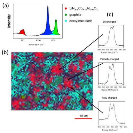
[24] | Lei J, McLarnon F, Kostecki R (2005) In situ Raman microscopy of individual LiNi0.8Co0.15Al0.05O2 particles in a Li-ion battery composite cathode. J Phys Chem B 109: 952–957. |
[25] |
Nakagawa H, Dom Yi, Doi T, et al. (2014) In situ Raman study of graphite negative-electrodes in electrolyte solution containing fluorinated phosphoric esters. J Electrochem Soc 161: A480–A485. doi: 10.1149/2.007404jes
![]() |
[26] |
Zhang X, Cheng F, Zhang K, et al. (2012) Facile polymer-assisted synthesis of LiNi0.5Mn1.5O4 with a hierarchical micro–nano structure and high rate capability. RSC Adv 2: 5669–5675. doi: 10.1039/C2RA20669B
![]() |
[27] |
Amaraj SF, Aurbach D (2011) The use of in situ techniques in R&D of Li and Mg rechargeable batteries. J Solid State Electr 15: 877–890. doi: 10.1007/s10008-011-1324-9
![]() |
[28] |
Stancovski V, Badilescu S (2014) In situ Raman spectroscopic–electrochemical studies of lithium-ion battery materials: a historical overview. J Appl Electrochem 44: 23–43. doi: 10.1007/s10800-013-0628-0
![]() |
[29] |
Baddour-Hadjean R, Pereira-Ramos JP (2010) Raman microspectrometry applied to the study of electrode materials for lithium batteries. Chem Rev 110: 1278–1319. doi: 10.1021/cr800344k
![]() |
[30] |
Burba CM, Frech R (2006) Modified coin cells for in situ Raman spectro-electrochemical measurements of LixV2O5 for lithium rechargeable batteries. Appl Spectrosc 60: 490–493. doi: 10.1366/000370206777412167
![]() |
[31] |
Gross T, Giebeler L, Hess C (2013) Novel in situ cell for Raman diagnostics of lithium-ion batteries. Rev Sci Instrum 84: 073109. doi: 10.1063/1.4813263
![]() |
[32] |
Gross T, Hess C (2014) Raman diagnostics of LiCoO2 electrodes for lithium-ion batteries. J Power Sources 256: 220–225. doi: 10.1016/j.jpowsour.2014.01.084
![]() |
[33] |
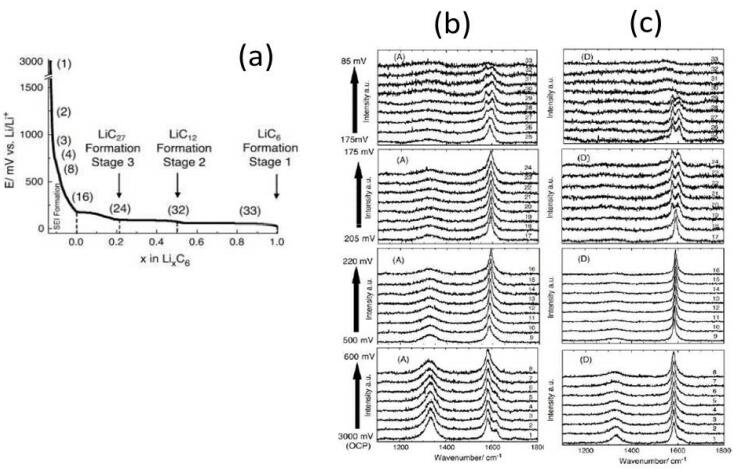
Sole C, Drewett NE, Hardwick LJ (2014) In situ Raman study of lithium-ion intercalation into microcrystalline graphite. Faraday Discuss 172: 223–237. doi: 10.1039/C4FD00079J
![]() |
[34] |
Novák P, Goers D, Hardwick L, et al. (2005) Advanced in situ characterization methods applied to carbonaceous materials. J Power Sources 146: 15–20. doi: 10.1016/j.jpowsour.2005.03.129
![]() |
[35] |
Fang S, Yan M, Hamers RJ (2017) Cell design and image analysis for in situ Raman mapping of inhomogeneous state-of-charge profiles in lithium-ion batteries. J Power Sources 352: 18–25. doi: 10.1016/j.jpowsour.2017.03.055
![]() |
[36] |
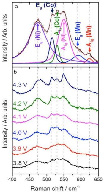
Ghanty C, Markovsky B, Erickson EM, et al. (2015) Li+-ion extraction/insertion of Ni-rich Li1+x(NiyCozMnz)wO2 (0.005 < x < 0.03; y:z = 8:1, w ≈ 1) electrodes: in situ XRD and Raman spectroscopy study. ChemElectroChem 2: 1479–1486. doi: 10.1002/celc.201500160
![]() |
[37] |
Huang JX, Li B, Liu B, et al. (2016) Structural evolution of NM (Ni and Mn) lithium-rich layered material revealed by in-situ electrochemical Raman spectroscopic study. J Power Sources 310: 85–90. doi: 10.1016/j.jpowsour.2016.01.065
![]() |
[38] |
Dash WC, Newman R (1955) Intrinsic optical absorption in single-crystal germanium and silicon at 77 K and 300 K. Phys Rev 99: 1151–1155. doi: 10.1103/PhysRev.99.1151
![]() |
[39] |
Brodsky MH, Title RS, Weiser K, et al. (1970) Structural, optical, and electrical properties of amorphous silicon films. Phys Rev B 1: 2632–2641. doi: 10.1103/PhysRevB.1.2632
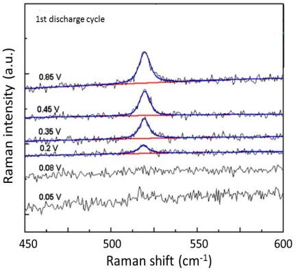
![]() |
[40] |
Pollak E, Salitra G, Baranchugov V, et al. (2007) In situ conductivity, impedance spectroscopy, and ex situ Raman spectra of amorphous silicon during the insertion/extraction of lithium. J Phys Chem C 111: 11437–11444. doi: 10.1021/jp0729563
![]() |
[41] |
Tuinstra F, Koenig JL (1970) Raman spectrum of graphite. J Chem Phys 53: 1126–1130. doi: 10.1063/1.1674108
![]() |
[42] |
Kostecki R, Schnyder B, Alliata D, et al. (2001) Surface studies of carbon films from pyrolyzed photoresist. Thin Solid Films 396: 36–43. doi: 10.1016/S0040-6090(01)01185-3
![]() |
[43] |
Julien CM, Zaghib K, Mauger A, et al. (2006) Characterization of the carbon coating onto LiFePO4 particles used in lithium batteries. J Appl Phys 100: 063511. doi: 10.1063/1.2337556
![]() |
[44] |
Panitz JC, Joho F, Novák P (1999) In situ characterization of a graphite electrode in a secondary lithium-ion battery using Raman microscopy. Appl Spectrosc 53: 1188–1199. doi: 10.1366/0003702991945650
![]() |
[45] |
Panitz JC, Novák P, Haas O (2001) Raman microscopy applied to rechargeable lithium-ion cells -Steps towards in situ Raman imaging with increased optical efficiency. Appl Spectrosc 55: 1131–1137. doi: 10.1366/0003702011953379
![]() |
[46] |
Panitz JC, Novák P (2001) Raman spectroscopy as a quality control tool for electrodes of lithium-ion batteries. J Power Sources 97–98: 174–180. doi: 10.1016/S0378-7753(01)00679-6
![]() |
[47] |
Kostecki R, Lei J, McLarnon F, et al. (2006) Diagnostic evaluation of detrimental phenomena in high-power lithium-ion batteries. J Electrochem Soc 153: A669–A672. doi: 10.1149/1.2170551
![]() |
[48] |
Forster JD, Harris SJ, Urban JJ (2014) Mapping Li+ concentration and transport via in situ confocal Raman microscopy. J Phys Chem Lett 5: 2007–2011. doi: 10.1021/jz500608e
![]() |
[49] |
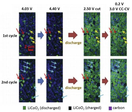
Nishi T, Nakai H, Kita A (2013) Visualization of the state-of-charge distribution in a LiCoO2 cathode by in situ Raman imaging. J Electrochem Soc 160: A1785–A1788. doi: 10.1149/2.061310jes
![]() |
[50] |
Nanda J, Remillard J, O'Neill A, et al. (2011) Local state-of-charge mapping of lithium-ion battery electrodes. Adv Funct Mater 21: 3282–3290. doi: 10.1002/adfm.201100157
![]() |
[51] |
Slautin B, Alikin D, Rosato D, et al. (2018) Local study of lithiation and degradation paths in LiMn2O4 battery cathodes: confocal Raman microscopy approach. Batteries 4: 21. doi: 10.3390/batteries4020021
![]() |
[52] |
Li J, Shunmugasundaram R, Doig R, et al. (2016) In situ X-ray diffraction study of layered Li–Ni–Mn–Co oxides: Effect of particle size and structural stability of core–shell materials. Chem Mater 28: 162–171. doi: 10.1021/acs.chemmater.5b03500
![]() |
[53] | Graetz J, Gabrisch H, Julien CM, et al. (2003) Raman evidence of spinel formation in delithiated cobalt oxide. Electrochemical society Proceedings Volume 2003-28; Proceedings-electrochemical Society PV, Symposium, Lithium and lithium-ion battery, 28: 95–100. |
[54] |
Yu L, Liu H, Wang Y, et al. (2013) Preferential adsorption of solvents on the cathode surface of lithium ion batteries. Angew Chem Int Edit 52: 5753–5756. doi: 10.1002/anie.201209976
![]() |
[55] | Kuwata N, Ise K, Matsuda Y, et al. (2012) Detection of degradation in LiCoO2 thin films by in situ micro Raman spectroscopy, In: Chowdari BVR, Kawamura J, Mizusaki J, et al. (Eds.), Solid State Ionics: Ionics for Sustainable World, Proceedings of the 13th Asian Conference, Singapore: World Scientific, 138–143. |
[56] |
Gross T, Hess C (2014) Spatially-resolved in situ Raman analysis of LiCoO2 electrodes. ECS Trans 61: 1–9. doi: 10.1149/06112.0001ecst
![]() |
[57] |
Fukumitsu H, Omori M, Terada K, et al. (2015) Development of in situ cross-sectional Raman imaging of LiCoO2 cathode for Li-ion battery. Electrochemistry 83: 993–996. doi: 10.5796/electrochemistry.83.993
![]() |
[58] |
Heber M, Schilling C, Gross T, et al. (2015) In situ Raman and UV-Vis spectroscopic analysis of lithium-ion batteries. MRS Proceedings 1773: 33–40. doi: 10.1557/opl.2015.634
![]() |
[59] |
Otoyama M, Ito Y, Hayashi A, et al. (2016) Raman imaging for LiCoO2 composite positive electrodes in all-solid-state lithium batteries using Li2S–P2S5 solid electrolytes. J Power Sources 302: 419–425. doi: 10.1016/j.jpowsour.2015.10.040
![]() |
[60] |
Porthault H, Baddour-Hadjean R, Le Cras F, et al. (2012) Raman study of the spinel-to-layered phase transformation in sol–gel LiCoO2 cathode powders as a function of the post-annealing temperature. Vib Spectrosc 62: 152–158. doi: 10.1016/j.vibspec.2012.05.004
![]() |
[61] |
Park Y, Kim NH, Kim JY, et al. (2010) Surface characterization of the high voltage LiCoO2/Li cell by X-ray photoelectron spectroscopy and 2D correlation analysis. Vib Spectrosc 53: 60–63. doi: 10.1016/j.vibspec.2010.01.004
![]() |
[62] |
Zhang X, Mauger A, Lu Q, et al. (2010) Synthesis and characterization of LiNi1/3Mn1/3Co1/3O2 by wet-chemical method. Electrochim Acta 55: 6440–6449. doi: 10.1016/j.electacta.2010.06.040
![]() |
[63] |
Ben-Kamel K, Amdouni N, Mauger A, et al. (2012) Study of the local structure of LiNi0.33+dMn0.33+dCo0.33−2dO2 (0.025 ≤ d ≤ 0.075) oxides. J Alloy Compd 528: 91–98. doi: 10.1016/j.jallcom.2012.03.018
![]() |
[64] | Hayden C, Talin AA (2014) Raman spectroscopic analysis of LiNi0.5Co0.2Mn0.3O2 cathodes stressed to high voltage. |
[65] |
Otoyama M, Ito Y, Hayashi A, et al. (2016) Raman spectroscopy for LiNi1/3Mn1/3Co1/3O2 composite positive electrodes in all-solid-state lithium batteries. Electrochemistry 84: 812–816. doi: 10.5796/electrochemistry.84.812
![]() |
[66] |
Lanz P, Villevieille C, Novák P (2014) Ex situ and in situ Raman microscopic investigation of the differences between stoichiometric LiMO2 and high-energy xLi2MnO3·(1 − x)LiMO2 (M = Ni, Co, Mn)· Electrochim Acta 130: 206–212. doi: 10.1016/j.electacta.2014.03.004
![]() |
[67] |
Koga H, Croguennec L, Mannessiez P, et al. (2012) Li1.20Mn0.54Co0.13Ni0.13O2 with different particle sizes as attractive positive electrode materials for lithium-ion batteries: Insights into their structure. J Phys Chem C 116: 13497–13506. doi: 10.1021/jp301879x
![]() |
[68] |
Julien CM, Massot M (2003) Lattice vibrations of materials for lithium rechargeable batteries III. Lithium manganese oxides. Mater Sci Eng B-Adv 100: 69–78. doi: 10.1016/S0921-5107(03)00077-1
![]() |
[69] |
Singh G, West WC, Soler J, et al. (2012) In situ Raman spectroscopy of layered solid solution Li2MnO3–LiMO2 (M = Ni, Mn, Co). J Power Sources 218: 34–38. doi: 10.1016/j.jpowsour.2012.06.083
![]() |
[70] |
Lanz P, Villevieille C, Novák P (2013) Electrochemical activation of Li2MnO3 at elevated temperature investigated by in situ Raman microscopy. Electrochim Acta 109: 426–432. doi: 10.1016/j.electacta.2013.07.130
![]() |
[71] |
Rao CV, Soler J, Katiyar R, et al. (2014) Investigations on electrochemical behavior and structural stability of Li1.2Mn0.54Ni0.13Co0.13O2 lithium-ion cathodes via in-situ and ex-situ Raman spectroscopy. J Phys Chem C 118: 14133–14141. doi: 10.1016/j.jpowsour.2014.10.032
![]() |
[72] |
Hy S, Felix F, Rick J, et al. (2014) Direct in situ observation of Li2O evolution on Li-rich high-capacity cathode material, Li[NixLi(1−2x)/3Mn(2−x)/3]O2 (0 ≤ x ≤ 0.5). J Am Chem Soc 136: 999–1007. doi: 10.1021/ja410137s
![]() |
[73] |
Shojan J, Rao-Chitturi V, Soler J, et al. (2015) High energy xLi2MnO3·(1 − x)LiNi2/3Co1/6Mn1/6O2 composite cathode for advanced Li-ion batteries.J Power Sources 274: 440–450. doi: 10.1016/j.jpowsour.2014.10.032
![]() |
[74] |
Grey CP, Yoon W, Reed J, et al. (2004) Electrochemical activity of Li in the transition-metal sites of O3 Li[Li (1−2x)/3Mn(2−x)/3Nix]O2. Electrochem Solid St 7: A290–A 293. doi: 10.1149/1.1783113
![]() |
[75] | Amalraj F, Talianker M, Markovsky B, et al. (2013) Study of the lithium-rich integrated compound xLi2MnO3·(1 − x)LiMO2 (x around 0.5; M = Mn, Ni, Co; 2:2:1) and its electrochemical activity as positive electrode in lithium cells. J Electrochem Soc 160: A324–A337. |
[76] |
Kumar-Nayak P, Grinblat J, Levi M, et al. (2014) Electrochemical and structural characterization of carbon coated Li1.2Mn0.56Ni0.16Co0.08O2 and Li1.2Mn0.6Ni0.2O2 as cathode materials for Li-ion batteries. Electrochim Acta 137: 546–556. doi: 10.1016/j.electacta.2014.06.055
![]() |
[77] |
Wu Q, Maroni VA, Gosztola DJ, et al. (2015) A Raman-based investigation of the fate of Li2MnO3 in lithium- and manganese-rich cathode materials for lithium ion batteries. J Electrochem Soc 162: A1255–A1264. doi: 10.1149/2.0631507jes
![]() |
[78] |
Bak SM, Nam KW, Chang W, et al. (2013) Correlating structure changes and gas evolution during the thermal decomposition of charged LixNi0.8Co0.15Al0.05O2 cathode material. Chem Mater 25: 337–351. doi: 10.1021/cm303096e
![]() |
[79] |
Julien C, Camacho-Lopez MA, Lemal M, et al. (2002) LiCo1−yMyO2 positive electrodes for rechargeable lithium batteries. I. Aluminum doped materials. Mater Sci Eng B-Adv 95: 6–13. doi: 10.1016/S0921-5107(01)01010-8
![]() |
[80] | Julien CM, Mauger A, Vijh A, et al. (2016) Cathode Materials with Monoatomic Ions in a Three-Dimensional Framework, In: Julien CM, Mauger A, Vijh A, et al., Lithium Batteries: Science and Technology, Cham, Switzerland: Springer, 163–199. |
[81] | Ohzuku T, Kitagawa M, Hirai T (1990) Electrochemistry of manganese dioxide in lithium nonaqueous cell. III. X-ray diffractional study on the reduction of spinel-related manganese dioxide. J Electrochem Soc 137: 769–775. |
[82] |
Liu W, Kowal K, Farrington GC (1998) Mechanism of the electrochemical insertion of lithium into LiMn2O4 spinels. J Electrochem Soc 145: 459–465. doi: 10.1149/1.1838285
![]() |
[83] |
Xia Y, Yoshio M (1996) An investigation of lithium ion insertion into spinel structure Li–Mn–O compounds. J Electrochem Soc 143: 825–833. doi: 10.1149/1.1836544
![]() |
[84] |
Richard MN, Keotschau I, Dahn JR (1997) A cell for in situ x‐ray diffraction based on coin cell hardware and Bellcore plastic electrode technology. J Electrochem Soc 144: 554–557. doi: 10.1149/1.1837447
![]() |
[85] | Yang XQ, Sun X, Lee SJ, et al. (1999) In situ synchrotron X‐ray diffraction studies of the phase transitions in LixMn2O4 cathode Materials. Electrochem Solid St 2: 157–160. |
[86] |
Kanamura K, Naito H, Yao T, et al. (1996) Structural change of the LiMn2O4 spinel structure induced by extraction of lithium. J Mater Chem 6: 33–36. doi: 10.1039/jm9960600033
![]() |
[87] |
White WB, DeAngelis A (1967) Interpretation of the vibrational spectra of spinels. Spectrochim Acta A 23: 985–995. doi: 10.1016/0584-8539(67)80023-0
![]() |
[88] |
Ammundsen B, Burns GR, Islam MS, et al. (1999) Lattice dynamics and vibrational spectra of lithium manganese oxides: A computer simulation and spectroscopic study. J Phys Chem B 103: 5175–5180. doi: 10.1021/jp984398l
![]() |
[89] | Kanoh H, Tang W, Ooi K (1998) In situ Raman spectroscopic study on electroinsertion of Li+ into a Pt/l-MnO2 electrode in aqueous solution. Electrochem Solid St 1: 17–19. |
[90] |
Huang W, Frech R (1999) In situ Raman spectroscopic studies of electrochemical intercalation in LixMn2O4-based cathodes. J Power Sources 81–82: 616–620. doi: 10.1016/S0378-7753(99)00231-1
![]() |
[91] |
Julien C, Massot M (2003) Lattice vibrations of materials for lithium rechargeable batteries I. Lithium manganese oxide spinel. Mater Sci Eng B-Adv 97: 217–230. doi: 10.1016/j.mseb.2003.09.028
![]() |
[92] |
Dokko K, Shi Q, Stefan IC, et al. (2003) In situ Raman spectroscopy of single microparticle Li+-intercalation electrodes. J Phys Chem B 107: 12549–12554. doi: 10.1021/jp034977c
![]() |
[93] |
Anzue N, Itoh T, Mohamedi M, et al. (2003) In situ Raman spectroscopic study of thin-film Li1−xMn2O4 electrodes. Solid State Ionics 156: 301–307. doi: 10.1016/S0167-2738(02)00693-8
![]() |
[94] |
Shi Q, Takahashi Y, Akimoto J, et al. (2005) In situ Raman scattering measurements of a LiMn2O4 single crystal microelectrode. Electrochem Solid St 8: A521–A524. doi: 10.1149/1.2030507
![]() |
[95] | Sun X, Yang XQ, Balasubramanian M, et al. (2002) In situ investigation of phase transitions of Li1+yMn2O4 spinel during Li-ion extraction and insertion. J Electrochem Soc 149: A842–A848. |
[96] |
Michalska M, Ziołkowska DA, Jasinski JB, et al. (2018) Improved electrochemical performance of LiMn2O4 cathode material by Ce doping. Electrochim Acta 276: 37–46. doi: 10.1016/j.electacta.2018.04.165
![]() |
[97] | Liu J, Manthiram A (2009) Understanding the improved electrochemical performances of Fe-substituted 5 V spinel cathode LiMn1.5Ni0.5O4. J Phys Chem C 113: 15073–15079. |
[98] |
Alcantara R, Jaraba M, Lavela P, et al. (2003) Structural and electrochemical study of new LiNi0.5TixMn1.5−xO4 spinel oxides for 5-V cathode materials. Chem Mater 15: 2376–2382. doi: 10.1021/cm034080s
![]() |
[99] | Zhong GB, Wang YY, Yu YQ, et al. (2012) Electrochemical investigations of the LiNi0.45M0.10Mn1.45O4 (M = Fe, Co, Cr) 5 V cathode materials for lithium ion batteries. J Power Sources 205: 385–393. |
[100] |
Liu D, Hamel-Paquet J, Trottier J, et al. (2012) Synthesis of pure phase disordered LiMn1.45Cr0.1Ni0.45O4 by a post-annealing method. J Power Sources 217: 400–406. doi: 10.1016/j.jpowsour.2012.06.063
![]() |
[101] |
Zhu W, Liu D, Trottier J, et al. (2014) Comparative studies of the phase evolution in M-doped LixMn1.5Ni0.5O4 (M = Co, Al, Cu and Mg) by in-situ X-ray diffraction. J Power Sources 264: 290–298. doi: 10.1016/j.jpowsour.2014.03.122
![]() |
[102] |
Dokko K, Mohamedi M, Anzue N, et al. (2002) In situ Raman spectroscopic studies of LiNixMn2−xO4 thin film cathode materials for lithium ion secondary batteries. J Mater Chem 12: 3688–3693. doi: 10.1039/B206764A
![]() |
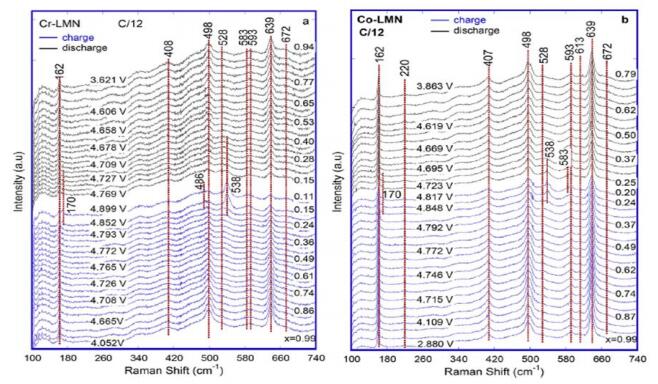
[103] | Zhu W, Liu D, Trottier J, et al. (2014) In situ Raman spectroscopic investigation of LiMn1.45Ni0.45M0.1O4 (M = Cr, Co) 5 V cathode materials. J Power Sources 298: 341–348. |
[104] |
Cocciantelli JM, Doumerc JP, Pouchard M, et al. (1991) Crystal chemistry of electrochemically inserted LixV2O5. J Power Sources 34: 103–111. doi: 10.1016/0378-7753(91)85029-V
![]() |
[105] | Zhang X, Frech R (1996) In situ Raman spectroscopy of LixV2O5 in a lithium rechargeable battery. ECS Proceedings 17: 198–203. |
[106] |
Baddour-Hadjean R, Navone C, Pereira-Ramos JP (2009) In situ Raman microspectrometry investigation of electrochemical lithium intercalation into sputtered crystalline V2O5 thin films. Electrochim Acta 54: 6674–6679. doi: 10.1016/j.electacta.2009.06.052
![]() |
[107] |
Jung H, Gerasopoulos K, Talin AA, et al. (2017) In situ characterization of charge rate dependent stress and structure changes in V2O5 cathode prepared by atomic layer deposition. J Power Sources 340: 89–97. doi: 10.1016/j.jpowsour.2016.11.035
![]() |
[108] |
Jung H, Gerasopoulos K, Talin AA, et al. (2017) A platform for in situ Raman and stress characterizations of V2O5 cathode using MEMS device. Electrochim Acta 242: 227–239. doi: 10.1016/j.electacta.2017.04.160
![]() |
[109] |
Julien C, Ivanov I, Gorenstein A (1995) Vibrational modifications on lithium intercalation in V2O5 films. Mater Sci Eng B-Adv 33: 168–172. doi: 10.1016/0921-5107(95)80032-8
![]() |
[110] |
Baddour-Hadjean R, Pereira-Ramos JP, Navone C, et al. (2008) Raman microspectrometry study of electrochemical lithium intercalation into sputtered crystalline V2O5 thin films. Chem Mater 20: 1916–1923. doi: 10.1021/cm702979k
![]() |
[111] |
Baddour-Hadjean R, Raekelboom E, Pereira-Ramos JP (2006) New structural characterization of the LixV2O5 system provided by Raman spectroscopy. Chem Mater 18: 3548–3556. doi: 10.1021/cm060540g
![]() |
[112] |
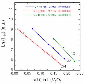
Baddour-Hadjean R, Marzouk A, Pereira-Ramos JP (2012) Structural modifications of LixV2O5 in a composite cathode (0 < x < 2) investigated by Raman microspectrometry. J Raman Spectrosc 43: 153–160. doi: 10.1002/jrs.2984
![]() |
[113] |
Baddour-Hadjean R, Pereira-Ramos JP (2007) New structural approach of lithium intercalation using Raman spectroscopy. J Power Sources 174: 1188–1192. doi: 10.1016/j.jpowsour.2007.06.177
![]() |
[114] |
Julien C, Massot M (2002) Spectroscopic studies of the local structure in positive electrodes for lithium batteries. Phys Chem Chem Phys 4: 4226–4235. doi: 10.1039/b203361e
![]() |
[115] |
Chen D, Ding D, Li X, et al. (2015) Probing the charge storage mechanism of a pseudocapacitive MnO2 electrode using in operando Raman spectroscopy. Chem Mater 27: 6608–6619. doi: 10.1021/acs.chemmater.5b03118
![]() |
[116] |
Julien CM, Massot M, Poinsignon C (2004) Lattice vibrations of manganese oxides: Part I. Periodic structures. Spectrochim Acta A 60: 689–700. doi: 10.1016/S1386-1425(03)00279-8
![]() |
[117] |
Hashem AM, Abuzeid H, Kaus M, et al. (2018) Green synthesis of nanosized manganese dioxide as positive electrode for lithium-ion batteries using lemon juice and citrus peel. Electrochim Acta 262: 74–81. doi: 10.1016/j.electacta.2018.01.024
![]() |
[118] |
Julien C, Massot M, Baddour-Hadjean R, et al. (2003) Raman spectra of birnessite manganese dioxides. Solid State Ionics 159: 345–356. doi: 10.1016/S0167-2738(03)00035-3
![]() |
[119] |
Hwang SJ, Park HS, Choy JH, et al. (2001) Micro-Raman spectroscopic study on layered lithium manganese oxide and its delithiated/relithiated derivatives. Electrochem Solid St 4: A213–A216. doi: 10.1149/1.1413704
![]() |
[120] |
Chen D, Ding D, Li X, et al. (2015) Probing the charge storage mechanism of a pseudocapacitive MnO2 electrode using in operando Raman spectroscopy. Chem Mater 27: 6608–6619. doi: 10.1021/acs.chemmater.5b03118
![]() |
[121] |
Yang L, Cheng S, Wang J, et al. (2016) Investigation into the origin of high stability of δ-MnO2 pseudo-capacitive electrode using operando Raman spectroscopy. Nano Energy 30: 293–302. doi: 10.1016/j.nanoen.2016.10.018
![]() |
[122] |
Zaghib K, Dontigny M, Perret P, et al. (2014) Electrochemical and thermal characterization of lithium titanate spinel anode in C-LiFePO4//C-Li4Ti5O12 cells at sub-zero temperatures. J Power Sources 248: 1050–1057. doi: 10.1016/j.jpowsour.2013.09.083
![]() |
[123] | Paques-Ledent MT, Tarte P (1974) Vibrational studies of olivine-type compounds 2. Orthophosphates, orthoarsenates and orthovanadates AIBIIXVO4. Spectrochim Acta A 30: 673–689. |
[124] | Wu J, Dathar GK, Sun C, et al. (2013) In situ Raman spectroscopy of LiFePO4: size and morphology dependence during charge and self-discharge. Nanotechnology 24: 424009. |
[125] |
Ramana CV, Mauger A, Gendron F, et al. (2009) Study of the Li-insertion/extraction process in LiFePO4/FePO4. J Power Sources 187: 555–564. doi: 10.1016/j.jpowsour.2008.11.042
![]() |
[126] |
Siddique NA, Salehi A, Wei Z, et al. (2015) Length‐scale‐dependent phase transformation of LiFePO4: An in situ and operando study using micro‐Raman spectroscopy and XRD. ChemPhysChem 16: 2383–2388. doi: 10.1002/cphc.201500299
![]() |
[127] |
Burba CM, Frech R (2004) Raman and FTIR spectroscopic study of LixFePO4 (0 ≤ x ≤ 1). J Electrochem Soc 151: A1032–A1038. doi: 10.1149/1.1756885
![]() |
[128] |
Morita M, Asai Y, Yoshimoto N, et al. (1998) A Raman spectroscopic study of organic electrolyte solutions based on binary solvent systems of ethylene carbonate with low viscosity solvents which dissolve different lithium salts. J Chem Soc Faraday Trans 94: 3451–3456. doi: 10.1039/a806278a
![]() |
[129] |
Burba CM, Frech R (2007) Vibrational spectroscopic studies of monoclinic and rhombohedral Li3V2(PO4)3. Solid State Ionics 177: 3445–3454. doi: 10.1016/j.ssi.2006.09.017
![]() |
[130] |
Yin SC, Grondey H, Strobel P, et al. (2003) Electrochemical property: Structure relationships in monoclinic Li3V2(PO4)3. J Am Chem Soc 125: 10402–10411. doi: 10.1021/ja034565h
![]() |
[131] | Takeuchi KJ, Marschilok AC, Davis SM, et al. (2001) Silver vanadium oxide and related battery applications. Coordin Chem Rev 219–221: 283–310. |
[132] |
Bao Q, Bao S, Li CM, et al. (2007) Lithium insertion in channel-structured b-AgVO3: in situ Raman study and computer simulation. Chem Mater 19: 5965–5972. doi: 10.1021/cm071728i
![]() |
[133] |
Tuinstra F, Koenig JL (1970) Raman spectrum of graphite. J Chem Phys 53: 1126–1130. doi: 10.1063/1.1674108
![]() |
[134] |
Reich S, Thomsen C (2004) Raman spectroscopy of graphite. Philos T R Soc A 362: 2271–2288. doi: 10.1098/rsta.2004.1454
![]() |
[135] |
Inaba M, Yoshida H, Yida H, et al. (1995) In situ Raman study on electrochemical Li intercalation into graphite. J Electrochem Soc 142: 20–26. doi: 10.1149/1.2043869
![]() |
[136] | Huang W, Frech R (1998) In situ Raman studies of graphite surface structures during lithium electrochemical intercalation. J Electrochem Soc 145: 765–770. |
[137] | Novák P, Joho F, Imhof R, et al. (1999) In situ investigation of the interaction between graphite and electrolyte solutions. J Power Sources 81–82: 212–216. |
[138] |
Luo Y, Cai WB, Scherson DA (2002) In situ, real-time Raman microscopy of embedded single particle graphite electrodes. J Electrochem Soc 149: A1100–A1105. doi: 10.1149/1.1492286
![]() |
[139] | Kostecki R, McLarnon F (2003) Microprobe study of the effect of Li intercalation on the structure of graphite. J Power Sources 119–121: 550–554. |
[140] |
Luo Y, Cai WB, Xing XK, et al. (2004) In situ, time-resolved Raman spectromicrotopography of an operating lithium-ion battery. Electrochem Solid St 7: E1–E5. doi: 10.1149/1.1627972
![]() |
[141] | Shi Q, Dokko K, Scherson DA (2004) In situ Raman microscopy of a single graphite microflake electrode in a Li+-containing electrolyte. J Phys Chem B 108: 4798–4793. |
[142] |
Migge S, Sandmann G, Rahner D, et al. (2005) Studying lithium intercalation into graphite particles via in situ Raman spectroscopy and confocal microscopy. J Solid State Electr 9: 132–137. doi: 10.1007/s10008-004-0563-4
![]() |
[143] |
Hardwick LJ, Hahn M, Ruch P, et al. (2006) Graphite surface disorder detection using in situ Raman microscopy. Solid State Ionics 177: 2801–2806. doi: 10.1016/j.ssi.2006.03.032
![]() |
[144] |
Hardwick LJ, Buqa H, Holzapfel M, et al. (2007) Behaviour of highly crystalline graphitic materials in lithium-ion cells with propylene carbonate containing electrolytes: An in situ Raman and SEM study. Electrochim Acta 52: 4884–4891. doi: 10.1016/j.electacta.2006.12.081
![]() |
[145] | Hardwick LJ, Marcinek M, Beer L, et al. (2008) An investigation of the effect of graphite degradation on irreversible capacity in lithium-ion cells. J Electrochem Soc 155: A442–A447. |
[146] |
Hardwick LJ, Ruch PW, Hahn M, et al. (2008) In situ Raman spectroscopy of insertion electrodes for lithium-ion batteries and supercapacitors: First cycle effects. J Phys Chem Solids 69: 1232–1237. doi: 10.1016/j.jpcs.2007.10.017
![]() |
[147] |
Nakagawa H, Ochida M, Domi Y, et al. (2012) Electrochemical Raman study of edge plane graphite negative-electrodes in electrolytes containing trialkyl phosphoric ester. J Power Sources 212: 148–153. doi: 10.1016/j.jpowsour.2012.04.013
![]() |
[148] | Underhill C, Leung SY, Dresselhaus G, et al. (1979) Infrared and Raman spectroscopy of graphite-ferric chloride. Solid State Commun 29: 769–774. |
[149] |
Hardwick LJ, Hahn M, Ruch P, et al. (2006) An in situ Raman study of the intercalation of supercapacitor-type electrolyte into microcrystalline graphite. Electrochim Acta 52: 675–680. doi: 10.1016/j.electacta.2006.05.053
![]() |
[150] | Solin SA (1990) Graphite Intercalation Compounds, Berlin: Springer-Verlag. |
[151] |
Brancolini G, Negri F (2004) Quantum chemical modeling of infrared and Raman activities in lithium-doped amorphous carbon nanostructures: hexa-peri-hexabenzocoronene as a model for hydrogen-rich carbon materials. Carbon 42: 1001–1005. doi: 10.1016/j.carbon.2003.12.016
![]() |
[152] |
Nakagawa H, Domi Y, Doi T, et al. (2012) In situ Raman study on degradation of edge plane graphite negative-electrodes and effects of film-forming additives. J Power Sources 206: 320–324. doi: 10.1016/j.jpowsour.2012.01.141
![]() |
[153] |
Perez-Villar S, Lanz P, Schneider H, et al. (2013) Characterization of a model solid electrolyte interphase/carbon interface by combined in situ Raman/Fourier transform infrared microscopy. Electrochim Acta 106: 506–515. doi: 10.1016/j.electacta.2013.05.124
![]() |
[154] |
Nakagawa H, Domi Y, Doi T, et al. (2013) In situ Raman study on the structural degradation of a graphite composite negative-electrode and the influence of the salt in the electrolyte solution. J Power Sources 236: 138–144. doi: 10.1016/j.jpowsour.2013.02.060
![]() |
[155] |
Lanz P, Novák P (2014) Combined in situ Raman and IR microscopy at the interface of a single graphite particle with ethylene carbonate/dimethyl carbonate. J Electrochem Soc 161: A1555–A1563. doi: 10.1149/2.0021410jes
![]() |
[156] |
Domi Y, Doi T, Nakagawa H, et al. (2016) In situ Raman study on reversible structural changes of graphite negative-electrodes at high potentials in LiPF6-Based electrolyte solution. J Electrochem Soc 163: A2435–A2440. doi: 10.1149/2.1301610jes
![]() |
[157] |
Yamanaka T, Nakagawa H, Tsubouchi S, et al. (2017) Correlations of concentration changes of electrolyte salt with resistance and capacitance at the surface of a graphite electrode in a lithium ion battery studied by in situ microprobe Raman spectroscopy. Electrochim Acta 251: 301–306. doi: 10.1016/j.electacta.2017.08.119
![]() |
[158] | Bhattacharya S, Alpas AT (2018) A novel elevated temperature pre-treatment for electrochemical capacity enhancement of graphene nanoflake-based anodes. Mater Renew Sustain Energy 7: 3. |
[159] |
Inaba M, Yoshida H, Ogumi Z (1996) In situ Raman study of electrochemical lithium insertion into mesocarbon microbeads heat‐treated at various temperatures. J Electrochem Soc 143: 2572–2578. doi: 10.1149/1.1837049
![]() |
[160] | Totir DA, Scherson DA (2000) Electrochemical and in situ Raman studies of embedded carbon particle electrodes in nonaqueous liquid electrolytes. Electrochem Solid St 3: 263–265. |
[161] |
Ramesha GK, Sampath S (2009) Electrochemical reduction of oriented graphene oxide films: an in situ Raman spectroelectrochemical study. J Phys Chem C 113: 7985–7989. doi: 10.1021/jp811377n
![]() |
[162] |
Tang W, Goh BM, Hu MY, et al. (2016) In situ Raman and nuclear magnetic resonance study of trapped lithium in the solid electrolyte interface of reduced graphene oxide. J Phys Chem C 120: 2600–2608. doi: 10.1021/acs.jpcc.5b12551
![]() |
[163] | Julien CM, Massot M, Zaghib K (2007) Structural studies of Li4/3Me5/3O4 (Me = Ti, Mn) electrode materials: local structure and electrochemical aspects. J Power Sources 136: 72–79. |
[164] |
Mukai K, Kato Y, Nakano H (2014) Understanding the zero-strain lithium insertion scheme of Li[Li1/3Ti5/3]O4: structural changes at atomic scale clarified by Raman spectroscopy. J Phys Chem C 118: 2992–2999. doi: 10.1021/jp412196v
![]() |
[165] |
Shu J, Shui M, Xu D, et al. (2011) Design and comparison of ex situ and in situ devices for Raman characterization of lithium titanate anode material. Ionics 17: 503–509. doi: 10.1007/s11581-011-0544-4
![]() |
[166] | Julien CM, Mauger A, Vijh A, et al. (2016) Anodes for Li-Ion Batteries, In: Julien CM, Mauger A, Vijh A, et al., Lithium Batteries: Science and Technology, Cham, Switzerland: Springer, 323–429. |
[167] |
Ohzuku T, Takehara Z, Yoshizawa S (1979) Non-aqueous lithium/titanium dioxide cell. Electrochim Acta 24: 219–222. doi: 10.1016/0013-4686(79)80028-6
![]() |
[168] | Wagemaker M, Borghols WJH, Mulder FM (2007) Large impact of particle size on insertion reactions. A case for anatase LixTiO2. J Am Chem Soc 129: 4323–4327. |
[169] |
Mukai K, Kato Y, Nakano H (2014) Understanding the zero-strain lithium insertion scheme of Li[Li1/3Ti5/3]O4: structural changes at atomic scale clarified by Raman spectroscopy. J Phys Chem C 118: 2992–2999. doi: 10.1021/jp412196v
![]() |
[170] |
Dinh NN, Oanh NTT, Long PD, et al. (2003) Electrochromic properties of TiO2 anatase thin films prepared by a dipping sol–gel method. Thin Solid Films 423: 70–76. doi: 10.1016/S0040-6090(02)00948-3
![]() |
[171] |
Smirnov M, Baddour-Hadjean R (2004) Li intercalation in TiO2 anatase: Raman spectroscopy and lattice dynamic studies. J Chem Phys 121: 2348–2355. doi: 10.1063/1.1767993
![]() |
[172] |
Baddour-Hadjean R, Bach S, Smirnov M, et al. (2004) Raman investigation of the structural changes in anatase LixTiO2 upon electrochemical lithium insertion. J Raman Spectrosc 35: 577–585. doi: 10.1002/jrs.1200
![]() |
[173] |
Hardwick LJ, Holzapfel M, Novák P, et al. (2007) Electrochemical lithium insertion into anatase-type TiO2: An in situ Raman microscopy investigation. Electrochim Acta 52: 5357–5367. doi: 10.1016/j.electacta.2007.02.050
![]() |
[174] |
Ren Y, Hardwick LJ, Bruce PG (2010) Lithium intercalation into mesoporous anatase with an ordered 3D pore structure. Angew Chem Int Edit 49: 2570–2574. doi: 10.1002/anie.200907099
![]() |
[175] |
Gentili V, Brutti S, Hardwick LJ, et al. (2012) Lithium insertion into anatase nanotubes. Chem Mater 24: 4468–4476. doi: 10.1021/cm302912f
![]() |
[176] |
Laskova BP, Frank O, Zukalova M, et al. (2013) Lithium insertion into titanium dioxide (anatase): A Raman study with 16/18O and 6/7Li isotope labeling. Chem Mater 25: 3710–3717. doi: 10.1021/cm402056j
![]() |
[177] |
Laskova BP, Kavan L, Zukalova M, et al. (2016) In situ Raman spectroelectrochemistry as a useful tool for detection of TiO2(anatase) impurities in TiO2(B) and TiO2(rutile). Monatsh Chem 147: 951–959. doi: 10.1007/s00706-016-1678-x
![]() |
[178] |
Mauger A, Xie H, Julien CM, (2016) Composite anodes for lithium-ion batteries, status and trends. AIMS Mater Sci 3: 1054–1106. doi: 10.3934/matersci.2016.3.1054
![]() |
[179] |
Li H, Huang X, Chen L, et al. (2000) The crystal structural evolution of nano-Si anode caused by lithium insertion and extraction at room temperature. Solid State Ionics 135: 181–191. doi: 10.1016/S0167-2738(00)00362-3
![]() |
[180] |
Nanda J, Datta MK, Remillard JT, et al. (2009) In situ Raman microscopy during discharge of a high capacity silicon–carbon composite Li-ion battery negative electrode. Electrochem Commun 11: 235–237. doi: 10.1016/j.elecom.2008.11.006
![]() |
[181] | Zeng Z, Liu N, Zeng Q, et al. (2016) In situ measurement of lithiation-induced stress in silicon nanoparticles using micro-Raman spectroscopy. Nano Energy 22: 105–110. |
[182] |
Tardif S, Pavlenko E, Quazuguel L, et al. (2017) Operando Raman spectroscopy and synchrotron X-ray diffraction of lithiation/delithiation in silicon nanoparticle anodes. ACS Nano 11: 11306–11316. doi: 10.1021/acsnano.7b05796
![]() |
[183] |
Miroshnikov Y, Zitoun D (2017) Operando plasmon-enhanced Raman spectroscopy in silicon anodes for Li-ion battery. J Nanopart Res 19: 372. doi: 10.1007/s11051-017-4063-8
![]() |
[184] |
Holzapfel M, Buqa H, Hardwick LJ, et al. (2006) Nano silicon for lithium-ion batteries. Electrochim Acta 52: 973–978. doi: 10.1016/j.electacta.2006.06.034
![]() |
[185] |
Long BR, Chan MKY, Greeley JP, et al. (2011) Dopant modulated Li insertion in Si for battery anodes: theory and experiment. J Phys Chem C 115: 18916–18921. doi: 10.1021/jp2060602
![]() |
[186] |
Miroshnikov Y, Yang J, Shokhen V, et al. (2018) Operando micro-Raman study revealing enhanced connectivity of plasmonic metals decorated silicon anodes for lithium-ion batteries. ACS Appl Energy Mater 1: 1096–1105. doi: 10.1021/acsaem.7b00220
![]() |
[187] | Zeng Z, Liu N, Zeng Q, et al. (2016) In situ measurement of lithiation-induced stress in silicon nanoparticles using micro-Raman spectroscopy. Nano Energy 22: 105–110. |
[188] |
Yang J, Kraytsberg A, Ein-Eli Y (2015) In situ Raman spectroscopy mapping of Si based anode material lithiation. J Power Sources 282: 294–298. doi: 10.1016/j.jpowsour.2015.02.044
![]() |
[189] |
Shimizu M, Usui H, Suzumura T, et al. (2015) Analysis of the deterioration mechanism of Si electrode as a Li-ion battery anode using Raman microspectroscopy. J Phys Chem C 119: 2975–2982. doi: 10.1021/jp5121965
![]() |
[190] |
Domi Y, Usui H, Shimizu M, et al. (2016) Effect of phosphorus-doping on electrochemical performance of silicon negative electrodes in lithium-ion batteries. ACS Appl Mater Inter 8: 7125–7132. doi: 10.1021/acsami.6b00386
![]() |
[191] |
Yamaguchi K, Domi Y, Usui H, et al. (2017) Elucidation of the reaction behavior of silicon negative electrodes in a bis(fluorosulfonyl)amide based ionic liquid electrolyte. ChemElectroChem 4: 3257–3263. doi: 10.1002/celc.201700724
![]() |
[192] |
Zhang WJ (2011) A review of the electrochemical performance of alloy anodes for lithium-ion batteries. J Power Sources 196: 13–24. doi: 10.1016/j.jpowsour.2010.07.020
![]() |
[193] |
Weppner W, Huggins RA (1977) Determination of the kinetic parameters of mixed-conducting electrodes and application to the system Li3Sb. J Electrochem Soc 124: 1569–1578. doi: 10.1149/1.2133112
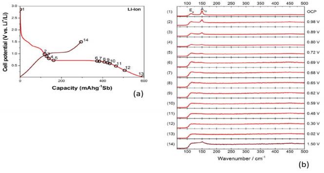
![]() |
[194] |
Drewett NE, Aldous AL, Zou J, et al. (2017) In situ Raman spectroscopic analysis of the lithiation and sodiation of antimony microparticles. Electrochim Acta 247: 296–305. doi: 10.1016/j.electacta.2017.07.030
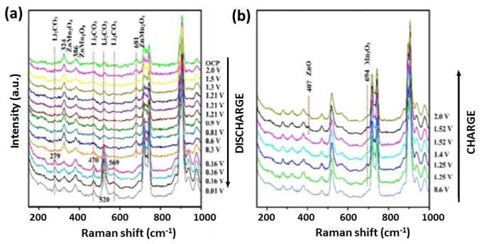
![]() |
[195] |
Zhong X, Wang X, Wang H, et al. (2018) Ultrahigh-performance mesoporous ZnMn2O4 microspheres as anode materials for lithium-ion batteries and their in situ Raman investigation. Nano Res 11: 3814. doi: 10.1007/s12274-017-1955-y
![]() |
[196] |
Cabo-Fernandez L, Mueller F, Passerini S, et al. (2016) In situ Raman spectroscopy of carbon-coated ZnFe2O4 anode material in Li-ion batteries-Investigation of SEI growth. Chem Commun 52: 3970–3973. doi: 10.1039/C5CC09350C
![]() |
[197] |
Schmitz R, Muller RA, Schmitz RW, et al. (2013) SEI investigations on copper electrodes after lithium plating with Raman spectroscopy and mass spectrometry. J Power Sources 233: 110–114. doi: 10.1016/j.jpowsour.2013.01.105
![]() |
[198] |
Hy S, Felix F, Chen YH, et al. (2014) In situ surface enhanced Raman spectroscopic studies of solid electrolyte interphase formation in lithium ion battery electrodes. J Power Sources 256: 324–328. doi: 10.1016/j.jpowsour.2014.01.092
![]() |
[199] | Yamanaka T, Nakagawa H, Tsubouchi S, et al. (2017) In situ diagnosis of the electrolyte solution in a laminate lithium ion battery by using ultrafine multi-probe Raman spectroscopy. J Power Sources 359: 435–440. |
[200] |
Yamanaka T, Nakagawa H, Tsubouchi S, et al. (2017) In situ Raman spectroscopic studies on concentration change of electrolyte salt in a lithium ion model battery with closely faced graphite composite and LiCoO2 composite electrodes by using an ultrafine microprobe. Electrochim Acta 234: 93–98. doi: 10.1016/j.electacta.2017.03.060
![]() |
[201] |
Yamanaka T , Nakagawa H, Tsubouchi S, et al. (2017) Effects of pored separator films at the anode and cathode sides on concentration changes of electrolyte salt in lithium ion batteries. Jpn J Appl Phys 56: 128002. doi: 10.7567/JJAP.56.128002
![]() |
[202] |
Naudin C, Bruneel JL, Chami M, et al. (2003) Characterization of the lithium surface by infrared and Raman spectroscopies. J Power Sources 124: 518–525. doi: 10.1016/S0378-7753(03)00798-5
![]() |
[203] |
Galloway TA, Cabo-Fernandez L, Aldous IM, et al. (2017) Shell isolated nanoparticles for enhanced Raman spectroscopy studies in lithium–oxygen cells. Faraday Discuss 205: 469–490. doi: 10.1039/C7FD00151G
![]() |
[204] |
Park Y, Kim Y, Kim SM, et al. (2017) Reaction at the electrolyte–electrode interface in a Li-ion battery studied by in situ Raman spectroscopy. Bull Korean Chem Soc 38: 511–513. doi: 10.1002/bkcs.11117
![]() |
[205] |
Yamanaka T, Nakagawa H, Tsubouchi S, et al. (2017) In situ Raman spectroscopic studies on concentration of electrolyte salt in lithium ion batteries by using ultrafine multifiber probes. ChemSusChem 10: 855–861. doi: 10.1002/cssc.201601473
![]() |
[206] | Lewis IR, Griffiths PR (1996) Raman spectrometry with fiber-optic sampling. Appl Spectrosc 50: 12A–30A. |
[207] |
Yamanaka T, Nakagawa H, Ochida M, et al. (2016) Ultrafine fiber Raman probe with high spatial resolution and fluorescence noise reduction. J Phys Chem C 120: 2585–2591. doi: 10.1021/acs.jpcc.5b11894
![]() |
[208] |
Yamanaka T, Nakagawa H, Tsubouchi S, et al. (2017) In situ Raman spectroscopic studies on concentration change of ions in the electrolyte solution in separator regions in a lithium ion battery by using multi-microprobes. Electrochem Commun 77: 32–35. doi: 10.1016/j.elecom.2017.01.020
![]() |
[209] |
Yamanaka T, Nakagawa H, Tsubouchi S, et al. (2017) Modification of the solid electrolyte interphase by chronoamperometric pretreatment and its effect on the concentration change of electrolyte salt in lithium ion batteries studied by in situ microprobe Raman spectroscopy. J Electrochem Soc 164: A2355–A2359. doi: 10.1149/2.0601712jes
![]() |
1. | Nikolai N. Nefedov, Lutz Recke, A common approach to singular perturbation and homogenization II: Semilinear elliptic systems, 2024, 0022247X, 129099, 10.1016/j.jmaa.2024.129099 |