Multiscale modeling, coarse-graining and shock wave computer simulations in materials science

Martin O. Steinhauser; Martin O. Steinhauser

doi:10.3934/matersci.2017.6.1319

AIMS Materials Science

2017, Volume 4, Issue 6: 1319-1357. doi: 10.3934/matersci.2017.6.1319

Previous Article Next Article

Review Topical Sections

Multiscale modeling, coarse-graining and shock wave computer simulations in materials science

Martin O. Steinhauser ^{1,2
,
,}

1.
Fraunhofer Institute for High-Speed Dynamics, Ernst-Mach-Institut, EMI, Eckerstrasse 4, 79104 Freiburg im Breisgau, Germany
2.
Department of Chemisty, Faculty of Science, University of Basel, Klingelbergstrasse 80, CH-4056 Basel, Switzerland

Received: 02 June 2017 Accepted: 03 September 2017 Published: 13 December 2017

My intention in this review article is to briefly discuss several major topics of presentday computational materials science in order to show their importance for state-of-the-art materials modeling and computer simulation. The topics I discuss are multiscale modeling approaches for hierarchical systems such as biological macromolecules and related coarse-graining techniques, which provide an efficient means to investigate systems on the mesoscale, and shock wave physics which has many important and interesting multi- and interdisciplinary applications in research areas where physics, biology, chemistry, computer science, medicine and even engineering meet. In fact, recently, as a new emerging field, the use of coarse-grained approaches for the simulation of biological macromolecules such as lipids and bilayer membranes and the investigation of their interaction with shock waves has become very popular. This emerging area of research may contribute not only to an improved understanding of the microscopic details of molecular self-assembly but may also lead to enhanced medical tumor treatments which are based on the destructive effects of High Intensity Focused Ultrasound (HIFU) or shock waves when interacting with biological cells and tissue; these are treatments which have been used in medicine for many years, but which are not well understood from a fundamental physical point of view.

Keywords:

Citation: Martin O. Steinhauser. Multiscale modeling, coarse-graining and shock wave computer simulations in materials science[J]. AIMS Materials Science, 2017, 4(6): 1319-1357. doi: 10.3934/matersci.2017.6.1319

Related Papers:

[1]	Mohammadjavad Hosseinpoor, Hamid Parvin, Samad Nejatian, Vahideh Rezaie, Karamollah Bagherifard, Abdollah Dehzangi, Amin Beheshti, Hamid Alinejad-Rokny . Proposing a novel community detection approach to identify cointeracting genomic regions. Mathematical Biosciences and Engineering, 2020, 17(3): 2193-2217. doi: 10.3934/mbe.2020117
[2]	Yue Hu, Xiaoqin Mei, Dong Tang . Long non-coding RNA XIST is down-regulated and correlated to better prognosis in ovarian cancer. Mathematical Biosciences and Engineering, 2020, 17(3): 2070-2081. doi: 10.3934/mbe.2020110
[3]	Ping Zhou, Yuting Zhang, Yunlei Yu, Weijia Cai, Guangquan Zhou . 3D shape measurement based on structured light field imaging. Mathematical Biosciences and Engineering, 2020, 17(1): 654-668. doi: 10.3934/mbe.2020034
[4]	Xiaohong Tian, Rui Xu, Jiazhe Lin . Mathematical analysis of an age-structured HIV-1 infection model with CTL immune response. Mathematical Biosciences and Engineering, 2019, 16(6): 7850-7882. doi: 10.3934/mbe.2019395
[5]	Choonsung Shin, Sung-Hee Hong, Hieyoung Jeong, Hyoseok Yoon, Byoungsoo Koh . All-in-one encoder/decoder approach for non-destructive identification of 3D-printed objects. Mathematical Biosciences and Engineering, 2022, 19(12): 14102-14115. doi: 10.3934/mbe.2022657
[6]	Sukun Tian, Ning Dai, Linlin Li, Weiwei Li, Yuchun Sun, Xiaosheng Cheng . Three-dimensional mandibular motion trajectory-tracking system based on BP neural network. Mathematical Biosciences and Engineering, 2020, 17(5): 5709-5726. doi: 10.3934/mbe.2020307
[7]	Ning Bai, Rui Xu . Mathematical analysis of an HIV model with latent reservoir, delayed CTL immune response and immune impairment. Mathematical Biosciences and Engineering, 2021, 18(2): 1689-1707. doi: 10.3934/mbe.2021087
[8]	Cuicui Cai, Maosheng Fu, Xianmeng Meng, Chaochuan Jia, Mingjing Pei . Indoor high-precision visible light positioning system using Jaya algorithm. Mathematical Biosciences and Engineering, 2023, 20(6): 10358-10375. doi: 10.3934/mbe.2023454
[9]	Xianfeng Xu, Liping Wang, Xiaohong Cheng, Weilin Ke, Shenqiu Jie, Shen Lin, Manlin Lai, Linlin Zhang, Zhenzhou Li . Machine learning-based evaluation of application value of the USM combined with NIPT in the diagnosis of fetal chromosomal abnormalities. Mathematical Biosciences and Engineering, 2022, 19(4): 4260-4276. doi: 10.3934/mbe.2022197
[10]	Xudan Ma, Qijun Zhang, Haihong Zhu, Kefeng Huang, Weina Pang, Qin Zhang . Establishment and analysis of the lncRNA-miRNA-mRNA network based on competitive endogenous RNA identifies functional genes in heart failure. Mathematical Biosciences and Engineering, 2021, 18(4): 4011-4026. doi: 10.3934/mbe.2021201

Abstract

References

[1]	Phillips RR (2001) Crystals, defects and microstructures: Modeling across scales, Cambridge: Cambridge University Press.
[2]	Yip S (2005) Handbook of materials modeling, Berlin: Springer.
[3]	Steinhauser MO (2017) Computational Multiscale Modeling of Fluids and Solids-Theory and Applications, 2nd Edition, Berlin: Springer.
[4]	McNeil PL, Terasaki M (2001) Coping with the inevitable: how cells repair a torn surface membrane. Nat Cell Biol 3: E124–E129. doi: 10.1038/35074652
[5]	Schmidt M, Kahlert U, Wessolleck J, et al. (2014) Characterization of a setup to test the impact of high-amplitude pressure waves on living cells. Sci Rep 4: 3849.
[6]	Gambihler S, Delius M, Ellwart JW (1992) Transient increase in membrane permeability of L1210 cells upon exposure to lithotripter shock waves in vitro. Naturwissenschaften 79: 328–329. doi: 10.1007/BF01138714
[7]	Gambihler S, Delius M, Ellwart JW (1994) Permeabilization of the plasma membrane of L1210 mouse leukemia cells using lithotripter shock waves. J Membrane Biol 141: 267–275.
[8]	Kodama T, Doukas AG, Hamblin MR (2002) Shock wave-mediated molecular delivery into cells. BBA-Mol Cell Res 1542: 186–194.
[9]	Bao G, Suresh S (2003) Cell and molecular mechanics of biological materials. Nat Mater 2: 715–725. doi: 10.1038/nmat1001
[10]	Tieleman DP, Leontiadou H, Mark AE, et al. (2003) Simulation of Pore Formation in Lipid Bilayers by Mechanical Stress and Electric Fields. J Am Chem Soc 125: 6382–6383. doi: 10.1021/ja029504i
[11]	Sundaram J, Mellein BR, Mitragotri S (2003) An Experimental and Theoretical Analysis of Ultrasound-Induced Permeabilization of Cell Membranes. Biophys J 84: 3087–3101. doi: 10.1016/S0006-3495(03)70034-4
[12]	Doukas AG, Kollias N (2004) Transdermal drug delivery with a pressure wave. Adv Drug Deliver Rev 56: 559–579. doi: 10.1016/j.addr.2003.10.031
[13]	Coussios CC, Roy RA (2008) Applications of Acoustics and Cavitation to Noninvasive Therapy and Drug Delivery. Annu Rev Fluid Mech 40: 395–420. doi: 10.1146/annurev.fluid.40.111406.102116
[14]	Prausnitz MR, Langer R (2008) Transdermal drug delivery. Nat Biotechnol 26: 1261–1268. doi: 10.1038/nbt.1504
[15]	Ashley CE, Carnes EC, Phillips GK, et al. (2011) The targeted delivery of multicomponent cargos to cancer cells by nanoporous particle-supported lipid bilayers. Nat Mater 10: 389–397. doi: 10.1038/nmat2992
[16]	Koshiyama K, Wada S (2011) Molecular dynamics simulations of pore formation dynamics during the rupture process of a phospholipid bilayer caused by high-speed equibiaxial stretching. J Biomech 44: 2053–2058. doi: 10.1016/j.jbiomech.2011.05.014
[17]	Steinhauser MO (2016) On the Destruction of Cancer Cells Using Laser-Induced Shock-Waves: A Review on Experiments and Multiscale Computer Simulations. Radiol Open J 1: 60–75. doi: 10.17140/ROJ-1-110
[18]	Krehl POK (2009) History of Shock Waves, Explosions and Impact: A Chronological and Biographical Reference, Berlin: Springer.
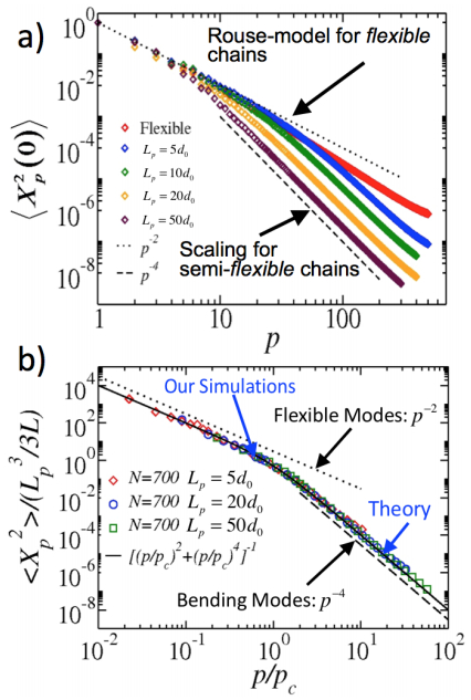
[19]	Steinhauser MO, Schneider J, Blumen A (2009) Simulating dynamic crossover behavior of semiflexible linear polymers in solution and in the melt. J Chem Phys 130: 164902. doi: 10.1063/1.3111038
[20]	Rodriguez V, Saurel R, Jourdan G, et al. (2013) Solid-particle jet formation under shock-wave acceleration. Phys Rev E 88: 063011. doi: 10.1103/PhysRevE.88.063011
[21]	Zheng J, Chen QF, Gu YJ, et al. (2012) Hugoniot measurements of double-shocked precompressed dense xenon plasmas. Phys Rev E 86: 066406. doi: 10.1103/PhysRevE.86.066406
[22]	Falk K, Regan SP, Vorberger J, et al. (2013) Comparison between x-ray scattering and velocityinterferometry measurements from shocked liquid deuterium. Phys Rev E 87: 043112. doi: 10.1103/PhysRevE.87.043112
[23]	Brujan EA, Matsumoto Y (2014) Shock wave emission from a hemispherical cloud of bubbles in non-Newtonian fluids. J Non-Newton Fluid 204: 32–37. doi: 10.1016/j.jnnfm.2013.12.003
[24]	Iakovlev S, Iakovlev S, Buchner C, et al. (2014) Resonance-like phenomena in a submerged cylindrical shell subjected to two consecutive shock waves: The effect of the inner fluid. J Fluid Struct 50: 153–170. doi: 10.1016/j.jfluidstructs.2014.05.013
[25]	Bringa EM, Caro A,Wang YM, et al. (2005) Ultrahigh strength in nanocrystalline materials under shock loading. Science 309: 1838–1841. doi: 10.1126/science.1116723
[26]	Kadau K, Germann TC, Lomdahl PS, et al. (2007) Shock waves in polycrystalline iron. Phys Rev Lett 98: 135701. doi: 10.1103/PhysRevLett.98.135701
[27]	Knudson MD, Desjarlais MP, Dolan DH (2008) Shock-Wave Exploration of the High-Pressure Phases of Carbon. Science 322: 1822–1825. doi: 10.1126/science.1165278
[28]	Gurnett DA, Kurth WS (2005) Electron plasma oscillations upstream of the solar wind termination shock. Science 309: 2025–2027. doi: 10.1126/science.1117425
[29]	Gurnett DA, Kurth WS (2008) Intense plasma waves at and near the solar wind termination shock. Nature 454: 78–80. doi: 10.1038/nature07023
[30]	Dutton Z, Budde M, Slowe C, et al. (2001) Observation of quantum shock waves created with ultra-compressed slow light pulses in a Bose-Einstein condensate. Science 293: 663–668. doi: 10.1126/science.1062527
[31]	Damski B (2006) Shock waves in a one-dimensional Bose gas: From a Bose-Einstein condensate to a Tonks gas. Phys Rev A 73: 043601. doi: 10.1103/PhysRevA.73.043601
[32]	Chang JJ, Engels P, Hoefer MA (2008) Formation of dispersive shock waves by merging and splitting Bose-Einstein condensates. Phys Rev Lett 101: 170404. doi: 10.1103/PhysRevLett.101.170404
[33]	Millot M, Dubrovinskaia N, Černok A, et al. (2015) Planetary science. Shock compression of stishovite and melting of silica at planetary interior conditions. Science 347: 418–420.
[34]	Bridge HS, Lazarus AJ, Snyder CW, et al. (1967) Mariner V: Plasma and Magnetic Fields Observed near Venus. Science 158: 1669–1673. doi: 10.1126/science.158.3809.1669
[35]	McKee CF, Draine BT (1991) Interstellar shock waves. Science 252: 397–403. doi: 10.1126/science.252.5004.397
[36]	McClure S, Dorfmüller C (2002) Extracorporeal shock wave therapy: Theory and equipment. Clin Tech Equine Pract 2: 348–357.
[37]	Lingeman JE, McAteer JA, Gnessin E, et al. (2009) Shock wave lithotripsy: advances in technology and technique. Nat Rev Urol 6: 660–670. doi: 10.1038/nrurol.2009.216
[38]	Cherenkov PA (1934) Visible emission of clean liquids by action of gamma radiation. Dokl Akad Nauk SSSR 2: 451–454.
[39]	Mach E, Salcher P (1887) Photographische Fixirung der durch Projectile in der Luft eingeleiteten Vorgänge. Ann Phys 268: 277–291. doi: 10.1002/andp.18872681008
[40]	Kühn M, Steinhauser MO (2008) Modeling and simulation of microstructures using power diagrams: Proof of the concept. Appl Phys Lett 93: 034102. doi: 10.1063/1.2959733
[41]	Walsh JM, Rice MH (1957) Dynamic compression of liquids from measurements on strong shock waves. J Chem Phys 26: 815–823. doi: 10.1063/1.1743414
[42]	Asay JR, Chhabildas LC (2003) Paradigms and Challenges in Shock Wave Research, High-Pressure Shock Compression of Solids VI, New York: Springer-Verlag New York, 57–119.
[43]	Steinhauser MO, Grass K, Strassburger E, et al. (2009) Impact failure of granular materials-Nonequilibrium multiscale simulations and high-speed experiments. Int J Plasticity 25: 161–182. doi: 10.1016/j.ijplas.2007.11.002
[44]	Watson E, Steinhauser MO (2017) Discrete Particle Method for Simulating Hypervelocity Impact Phenomena. Materials 10: 379. doi: 10.3390/ma10040379
[45]	Holian BL, Lomdahl PS (1998) Plasticity induced by shock waves in nonequilibrium moleculardynamics simulations. Science 280: 2085–2088. doi: 10.1126/science.280.5372.2085
[46]	Kadau K, Germann TC, Lomdahl PS, et al. (2002) Microscopic view of structural phase transitions induced by shock waves. Science 296: 1681–1684. doi: 10.1126/science.1070375
[47]	Chen M, McCauley JW, Hemker KJ (2003) Shock-Induced Localized Amorphization in Boron Carbide. Science 299: 1563–1566. doi: 10.1126/science.1080819
[48]	Holian BL (2004) Molecular dynamics comes of age for shockwave research. Shock Waves 13: 489–495.
[49]	Germann TC, Kadau K (2008) Trillion-atom molecular dynamics becomes a reality. Int J Mod Phys C 19: 1315–1319. doi: 10.1142/S0129183108012911
[50]	Ciccotti G, Frenkel G, McDonald IR (1987) Simulation of Liquids and Solids, Amsterdam: North-Holland.
[51]	Allen MP, Tildesley DJ (1987) Computer Simulation of Liquids, Oxford, UK: Clarendon Press.
[52]	Liu WK, Hao S, Belytschko T, et al. (1999) Multiple scale meshfree methods for damage fracture and localization. Comp Mater Sci 16: 197–205. doi: 10.1016/S0927-0256(99)00062-2
[53]	Gates TS, Odegard GM, Frankland SJV, et al. (2005) Computational materials: Multi-scale modeling and simulation of nanostructured materials. Compos Sci Technol 65: 2416–2434. doi: 10.1016/j.compscitech.2005.06.009
[54]	Steinhauser MO (2013) Computer Simulation in Physics and Engineering, 1st Edition, Berlin: deGruyter.
[55]	Finnis MW, Sinclair JE (1984) A simple empirical N-body potential for transition metals. Philos Mag A 50: 45–55. doi: 10.1080/01418618408244210
[56]	Kohn W (1996) Density functional and density matrix method scaling linearly with the number of atoms. Phys Rev Lett 76: 3168–3171. doi: 10.1103/PhysRevLett.76.3168
[57]	Car R, Parrinello M (1985) Unified approach for molecular dynamics and density-functional theory. Phys Rev Lett 55: 2471–2474. doi: 10.1103/PhysRevLett.55.2471
[58]	Elstner M, Porezag D, Jungnickel G, et al. (1998) Self-consistent-charge density-functional tightbinding method for simulations of complex materials properties. Phys Rev B 58: 7260–7268. doi: 10.1103/PhysRevB.58.7260
[59]	Sutton AP, Finnis MW, Pettifor DG, et al. (1988) The tight-binding bond model. J Phys C-Solid State Phys 21: 35–66. doi: 10.1088/0022-3719/21/1/007
[60]	Szabo A, Ostlund NS (1996) Modern quantum chemistry: introduction to advanced electronic structure theory, (Dover Books on Chemistry), New York: Dover Publications.
[61]	Kadau K, Germann TC, Lomdahl PS (2006) Molecular dynamics comes of age: 320 billion atom simulation on BlueGene/L. Int J Mod Phys C 17: 1755–1761. doi: 10.1142/S0129183106010182
[62]	Fineberg J (2003) Materials science: close-up on cracks. Nature 426: 131–132. doi: 10.1038/426131a
[63]	Buehler M, Hartmaier A, Gao H, et al. (2004) Atomic plasticity: description and analysis of a onebillion atom simulation of ductile materials failure. Comput Method Appl M 193: 5257–5282. doi: 10.1016/j.cma.2003.12.066
[64]	Abraham FF, Gao HJ (2000) How fast can cracks propagate? Phys Rev Lett 84: 3113–3116. doi: 10.1103/PhysRevLett.84.3113
[65]	Bulatov V, Abraham FF, Kubin L, et al. (1998) Connecting atomistic and mesoscale simulations of crystal plasticity. Nature 391: 669–672. doi: 10.1038/35577
[66]	Gross SP, Fineberg J, Marder M, et al. (1993) Acoustic emissions from rapidly moving cracks. Phys Rev Lett 71: 3162–3165. doi: 10.1103/PhysRevLett.71.3162
[67]	Courant R (1943) Variational Methods for the Solution of Problems of Equilibrium and Vibrations. B Am Math Soc 49: 1–23.
[68]	Lucy LB (1977) A numerical approach to the testing of the fission hypothesis. Astron J 82: 1013–1024. doi: 10.1086/112164
[69]	Cabibbo N, Iwasaki Y, Schilling K (1999) High performance computing in lattice QCD. Parallel Comput 25: 1197–1198. doi: 10.1016/S0167-8191(99)00045-9
[70]	Evertz HG (2003) The loop algorithm. Adv Phys 52: 1–66. doi: 10.1080/0001873021000049195
[71]	Holm EA, Battaile CC (2001) The computer simulation of microstructural evolution. JOM 53: 20–23.
[72]	Nielsen SO, Lopez CF, Srinivas G, et al. (2004) Coarse grain models and the computer simulation of soft materials. J Phys-Condens Mat 16: 481–512. doi: 10.1088/0953-8984/16/15/R03
[73]	Praprotnik M, Site LD, Kremer K (2008) Multiscale simulation of soft matter: From scale bridging to adaptive resolution. Annu Rev Phys Chem 59: 545–571. doi: 10.1146/annurev.physchem.59.032607.093707
[74]	Karimi-Varzaneh HA, Müller-Plathe F (2011) Coarse-Grained Modeling for Macromolecular Chemistry, In: Kirchner B, Vrabec J, Topics in Current Chemistry, Berlin, Heidelberg: Springer, 326–321.
[75]	Müller-Plathe F (2002) Coarse-graining in polymer simulation: from the atomistic to the mesoscopic scale and back. Chem Phys Chem 3: 755–769.
[76]	Abraham FF, Broughton JQ, Broughton JQ, et al. (1998) Spanning the length scales in dynamic simulation. Comp Phys 12: 538–546. doi: 10.1063/1.168756
[77]	Abraham FF, Brodbeck D, Rafey R, et al. (1994) Instability dynamics of fracture: A computer simulation investigation. Phys Rev Lett 73: 272–275. doi: 10.1103/PhysRevLett.73.272
[78]	Abraham FF, Brodbeck D, Rudge WE, et al. (1998) Ab initio dynamics of rapid fracture. Model Simul Mater Sc 6: 639–670. doi: 10.1088/0965-0393/6/5/010
[79]	Warshel A, LevittM(1976) Theoretical studies of enzymic reactions: Dielectric, electrostatic and steric stabilization of the carbonium ion in the reaction of lysozyme. J Mol Biol 103: 227–249.
[80]	Winkler RG, Steinhauser MO, Reineker P (2002) Complex formation in systems of oppositely charged polyelectrolytes: a molecular dynamics simulation study. Phys Rev E 66: 021802.
[81]	Dünweg B, Reith D, Steinhauser M, et al. (2002) Corrections to scaling in the hydrodynamic properties of dilute polymer solutions. J Chem Phys 117: 914–924. doi: 10.1063/1.1483296
[82]	Stevens MJ (2004) Coarse-grained simulations of lipid bilayers. J Chem Phys 121: 11942–11948. doi: 10.1063/1.1814058
[83]	Steinhauser MO (2005) A molecular dynamics study on universal properties of polymer chains in different solvent qualities. Part I. A review of linear chain properties. J Chem Phys 122: 094901.
[84]	Steinhauser MO, Hiermaier S (2009) A Review of Computational Methods in Materials Science: Examples from Shock-Wave and Polymer Physics. Int J Mol Sci 10: 5135–5216. doi: 10.3390/ijms10125135
[85]	Goetz R, Gompper G, Lipowsky R (1999) Mobility and elasticity of self-assembled membranes. Phys Rev Lett 82: 221–224. doi: 10.1103/PhysRevLett.82.221
[86]	Lipowsky R (2004) Biomimetic membrane modelling: pictures from the twilight zone. Nat Mater 3: 589–591. doi: 10.1038/nmat1208
[87]	Lyubartsev AP (2005) Multiscale modeling of lipids and lipid bilayers. Eur Biophys J 35: 53–61. doi: 10.1007/s00249-005-0005-y
[88]	Orsi M, Michel J, Essex JW (2010) Coarse-grain modelling of DMPC and DOPC lipid bilayers. J Phys-Condens Mat 22: 155106. doi: 10.1088/0953-8984/22/15/155106
[89]	Steinhauser MO (2012) Introduction to Molecular Dynamics Simulations: Applications in Hard and Soft Condensed Matter Physics, InTech.
[90]	Alberts B, Bray D, Johnson A, et al. (2000) Molecular Biology of the Cell, 4 Edition, New York: Garland Science, Taylor and Francis Group.
[91]	Steinhauser MO, Steinhauser MO, Schmidt M (2014) Destruction of cancer cells by laserinduced shock waves: recent developments in experimental treatments and multiscale computer simulations. Soft Matter 10: 4778–4788. doi: 10.1039/C4SM00407H
[92]	Tozzini V (2004) Coarse-grained models for proteins. Curr Opin Struc Biol 15: 144–150.
[93]	Ayton GS, Noid WG, Voth GA (2007) Multiscale modeling of biomolecular systems: in serial and in parallel. Curr Opin Struc Biol 17: 192–198. doi: 10.1016/j.sbi.2007.03.004
[94]	Forrest LR, Sansom MS (2000) Membrane simulations: bigger and better? Curr Opin Struc Biol 10: 174–181. doi: 10.1016/S0959-440X(00)00066-X
[95]	Woods CJ, Mulholland AJ (2008) Multiscale modelling of biological systems. RSC Special Periodicals Report: Chemical Modelling, Applications and Theory 5: 13–50. doi: 10.1039/b608778g
[96]	Steinhauser MO (editor) (2016) Special Issue of the Journal Materials: Computational Multiscale Modeling and Simulation in Materials Science. Available from: http://www.mdpi.com/journal/materials/special issues/modeling and simulation.
[97]	Brendel W (1986) Shock Waves: A New Physical Principle in Medicine. Eur Surg Res 18: 177–180. doi: 10.1159/000128523
[98]	Wang CJ (2003) An overview of shock wave therapy in musculoskeletal disorders. Chang Gung Med J 26: 220–232.
[99]	Wang ZJZ, DesernoM (2010) A systematically coarse-grained solvent-free model for quantitative phospholipid bilayer simulations. J Phys Chem B 114: 11207–11220. doi: 10.1021/jp102543j
[100]	Wang ZB, Wu J, Fang LQ, et al. (2011) Preliminary ex vivo feasibility study on targeted cell surgery by high intensity focused ultrasound (HIFU). Ultrasonics 51: 369–375. doi: 10.1016/j.ultras.2010.11.002
[101]	Wang S, Frenkel V, Zderic V (2011) Optimization of pulsed focused ultrasound exposures for hyperthermia applications. J Acoust Soc Am 130: 599–609. doi: 10.1121/1.3598464
[102]	Paul W, Smith GD, Yoon DY (1997) Static and dynamic properties of an-C100H202 melt from molecular dynamics simulations. Macromolecules 30: 7772–7780. doi: 10.1021/ma971184d
[103]	Kreer T, Baschnagel J, Mueller M, et al. (2001) Monte Carlo Simulation of long chain polymer melts: Crossover from Rouse to reptation dynamics. Macromolecules 34: 1105–1117. doi: 10.1021/ma001500f
[104]	Krushev S, Paul W, Smith GD (2002) The role of internal rotational barriers in polymer melt chain dynamics. Macromolecules 35: 4198–4203. doi: 10.1021/ma0115794
[105]	Bulacu M, van der Giessen E (2005) Effect of bending and torsion rigidity on self-diffusion in polymer melts: A molecular-dynamics study. J Chem Phys 123: 114901. doi: 10.1063/1.2035086
[106]	Kratky O, Porod G (1949) Röntgenuntersuchung gelöster Fadenmoleküle. Recl Trva Chim Pays-Bas 68: 1106–1122.
[107]	Doi M, Edwards SF (1986) The Theory of Polymer Dynamics, Oxford: Clarendon Press.
[108]	Harris RA, Hearst JE (1966) On Polymer Dynamics. J Chem Phys 44: 2595–2602. doi: 10.1063/1.1727098
[109]	Hearst JE, Harris RA (1967) On Polymer Dynamics. III. Elastic Light Scattering. J Chem Phys 46: 398–398.
[110]	Harnau L, Winkler RG, Reineker P (1997) Influence of stiffness on the dynamics of macromolecules in a melt. J Chem Phys 106: 2469–2476. doi: 10.1063/1.473154
[111]	Harnau L, WInkler RG, Reineker P (1999) On the dynamics of polymer melts: Contribution of Rouse and bending modes. EPL 45: 488–494. doi: 10.1209/epl/i1999-00193-6
[112]	Steinhauser MO (2008) Static and dynamic scaling of semiflexible polymer chains-a molecular dynamics simulation study of single chains and melts. Mech Time-Depend Mat 12: 291–312. doi: 10.1007/s11043-008-9062-9
[113]	Guenza M (2003) Cooperative dynamics in semiflexibile unentangled polymer fluids. J Chem Phys 119: 7568–7578. doi: 10.1063/1.1606674
[114]	Piran T (2004) Statistical Mechanics of Membranes and Interfaces, 2 edition, World Scientific Publishing Co., Inc.
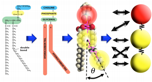
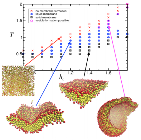
[115]	Schindler T, Kröner D, Steinhauser MO (2016) On the dynamics of molecular self-assembly and the structural analysis of bilayer membranes using coarse-grained molecular dynamics simulations. BBA-Biomembranes 1858: 1955–1963. doi: 10.1016/j.bbamem.2016.05.014
[116]	Brannigan G, Lin LCL, Brown FLH (2006) Implicit solvent simulation models for biomembranes. Eur Biophys J 35: 104–124. doi: 10.1007/s00249-005-0013-y
[117]	Chang R, Ayton GS, Voth GA (2005) Multiscale coupling of mesoscopic- and atomistic-level lipid bilayer simulations. J Chem Phys 122: 244716. doi: 10.1063/1.1931651
[118]	Huang MJ, Kapral R, Mikhailov AS, et al. (2012) Coarse-grain model for lipid bilayer selfassembly and dynamics: Multiparticle collision description of the solvent. J Chem Phys 137: 055101. doi: 10.1063/1.4736414
[119]	Pandit SA, Scott HL (2009) Multiscale simulations of heterogeneous model membranes. BBA-Biomembranes 1788: 136–148. doi: 10.1016/j.bbamem.2008.09.004
[120]	Farago O (2003) "Water-free" computer model for fluid bilayer membranes. J Chem Phys 119: 596–605. doi: 10.1063/1.1578612
[121]	Brannigan G, Philips PF, Brown FLH (2005) Flexible lipid bilayers in implicit solvent. Phys Rev E 72: 011915. doi: 10.1103/PhysRevE.72.011915
[122]	Yuan H, Huang C, Li J, et al. (2010) One-particle-thick, solvent-free, coarse-grained model for biological and biomimetic fluid membranes. Phys Rev E 82: 011905. doi: 10.1103/PhysRevE.82.011905
[123]	Noguchi H (2011) Solvent-free coarse-grained lipid model for large-scale simulations. J Chem Phys 134: 055101. doi: 10.1063/1.3541246
[124]	Weiner SJ, Kollman PA, Case DA, et al. (1984) A new force field for molecular mechanical simulation of nucleic acids and proteins. J Am Chem Soc 106: 765–784. doi: 10.1021/ja00315a051
[125]	Paul W, Yoon DY, Smith GD, et al. (1995) An Optimized United Atom Model for Simulations of Polymethylene Melts. J Chem Phys 103: 1702–1709. doi: 10.1063/1.469740
[126]	Siu SWI, Vácha R, Jungwirth P, et al. (2008) Biomolecular simulations of membranes: physical properties from different force fields. J Phys Chem 128: 125103. doi: 10.1063/1.2897760
[127]	Drouffe JM, Maggs AC, Leibler S, et al. (1991) Computer simulations of self-assembled membranes. Science 254: 1353–1356. doi: 10.1126/science.1962193
[128]	Goetz R, Lipowsky R (1998) Computer simulations of bilayer membranes: Self-assembly and interfacial tension. J Chem Phys 108: 7397–7409. doi: 10.1063/1.476160
[129]	Noguchi H, Takasu M (2001) Self-assembly of amphiphiles into vesicles: A Brownian dynamics simulation. Phys Rev E 64: 041913. doi: 10.1103/PhysRevE.64.041913
[130]	Bourov GK, Bhattacharya A (2005) Brownian dynamics simulation study of self-assembly of amphiphiles with large hydrophilic heads. J Chem Phys 122: 44702. doi: 10.1063/1.1834495
[131]	Steinhauser MO, Grass K, Thoma K, et al. (2006) Impact dynamics and failure of brittle solid states by means of nonequilibrium molecular dynamics simulations. EPL 73: 62–68. doi: 10.1209/epl/i2005-10353-2
[132]	Yang S, Qu J (2014) Coarse-grained molecular dynamics simulations of the tensile behavior of a thermosetting polymer. Phys Rev E 90: 012601. doi: 10.1103/PhysRevE.90.012601
[133]	Eslami H, Müller-Plathe F (2013) How thick is the interphase in an ultrathin polymer film? Coarse-grained molecular dynamics simulations of polyamide-6,6 on graphene. J Phys Chem 117: 5249–5257.
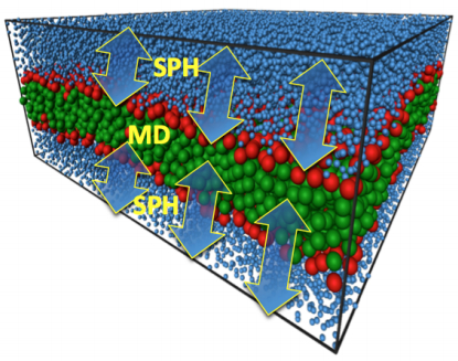
[134]	Ganzenm¨uller GC, Hiermaier S, Steinhauser MO (2011) Shock-wave induced damage in lipid bilayers: a dissipative particle dynamics simulation study. Soft Matter 7: 4307–4317. doi: 10.1039/c0sm01296c
[135]	Huang WX, Chang CB, Sung HJ (2012) Three-dimensional simulation of elastic capsules in shear flow by the penalty immersed boundary method. J Comput Phys 231: 3340–3364. doi: 10.1016/j.jcp.2012.01.006
[136]	Pazzona FG, Demontis P (2012) A grand-canonical Monte Carlo study of the adsorption properties of argon confined in ZIF-8: local thermodynamic modeling. J Phys Chem 117: 349–357.
[137]	Pogodin S, Baulin VA (2010) Coarse-grained models of phospholipid membranes within the single chain mean field theory. Soft Matter 6: 2216–2226. doi: 10.1039/b927437e
[138]	Wang Y, Sigurdsson JK, Brandt E, et al. (2013) Dynamic implicit-solvent coarse-grained models of lipid bilayer membranes: fluctuating hydrodynamics thermostat. Phys Rev E 88: 023301. doi: 10.1103/PhysRevE.88.023301
[139]	Koshiyama K, Kodama T, Yano T, et al. (2006) Structural Change in Lipid Bilayers and Water Penetration Induced by Shock Waves: Molecular Dynamics Simulations. Biophys J 91: 2198–2205. doi: 10.1529/biophysj.105.077677
[140]	Koshiyama K, Kodama T, Yano T, et al. (2008) Molecular dynamics simulation of structural changes of lipid bilayers induced by shock waves: Effects of incident angles. BBA-Biomembranes 1778: 1423–1428. doi: 10.1016/j.bbamem.2008.03.010
[141]	Lechuga J, Drikakis D, Pal S (2008) Molecular dynamics study of the interaction of a shock wave with a biological membrane. Int J Numer Mech Fluids 57: 677–692. doi: 10.1002/fld.1588
[142]	Kodama T, Kodama T, Hamblin MR, et al. (2000) Cytoplasmic molecular delivery with shock waves: importance of impulse. Biophys J 79: 1821–1832. doi: 10.1016/S0006-3495(00)76432-0
[143]	Doukas AG, McAuliffe DJ, Lee S, et al. (1995) Physical factors involved in stress-wave-induced cell injury: The effect of stress gradient. Ultrasound Med Biol 21: 961–967. doi: 10.1016/0301-5629(95)00027-O
[144]	Doukas AG, Flotte TJ (1996) Physical characteristics and biological effects of laser-induced stress waves. Ultrasound Med Biol 22: 151–164. doi: 10.1016/0301-5629(95)02026-8
[145]	Lee S, Doukas AG (1999) Laser-generated stress waves and their effects on the cell membrane. IEEE J Sel Top Quant 5: 997–1003. doi: 10.1109/2944.796322
[146]	Español P (1997) Dissipative Particle Dynamics with energy conservation. EPL 40: 631–636. doi: 10.1209/epl/i1997-00515-8
[147]	Steinhauser MO, Schindler T (2017) Particle-based simulations of bilayer membranes: selfassembly, structural analysis, and shock-wave damage. Comp Part Mech 4: 69–86. doi: 10.1007/s40571-016-0126-3
[148]	Hansen JP, McDonald IR (2005) Theory of Simple Liquids, Academic Press.

This article has been cited by:

1.	Palle E. T. Jorgensen, Unbounded graph-Laplacians in energy space, and their extensions, 2012, 39, 1598-5865, 155, 10.1007/s12190-011-0518-8
2.	Joachim von Below, José A. Lubary, Baptiste Vasseur, Some Remarks on the Eigenvalue Multiplicities of the Laplacian on Infinite Locally Finite Trees, 2013, 63, 1422-6383, 1331, 10.1007/s00025-012-0271-9
3.	Joachim Kerner, Matthias Täufer, Jens Wintermayr, Robustness of Flat Bands on the Perturbed Kagome and the Perturbed Super-Kagome Lattice, 2023, 1424-0637, 10.1007/s00023-023-01399-7

Reader Comments

Your name:*

Email:*
© 2017 the Author(s), licensee AIMS Press. This is an open access article distributed under the terms of the Creative Commons Attribution License (http://creativecommons.org/licenses/by/4.0)