Evaluation of effective hyperelastic material coefficients for multi-defected solids under large deformation

Jui-Hung Chang; Weihan Wu; Jui-Hung Chang; Weihan Wu

doi:10.3934/matersci.2016.4.1773

AIMS Materials Science

2016, Volume 3, Issue 4: 1773-1795. doi: 10.3934/matersci.2016.4.1773

Previous Article Next Article

Research article Special Issues

Evaluation of effective hyperelastic material coefficients for multi-defected solids under large deformation

Jui-Hung Chang ^{1
,
,},
Weihan Wu ²

1.
Department of Civil Engineering, National Central University, Zhongli, Taoyuan 32001, Taiwan
2.
Department of Mathematics, National Central University, Zhongli, Taoyuan 32001, Taiwan

Received: 07 August 2016 Accepted: 10 November 2016 Published: 09 December 2016

The present work deals with the modeling of multi-defected solids under the action of large deformation. A micromechanics constitutive model, formulated in terms of the compressible anisotropic NeoHookean strain energy density function, is presented to characterize the corresponding nonlinear effective elastic behavior. By employing a scalar energy parameter, a correspondence relation between the effective hyperelastic model and this energy parameter is established. The corresponding effective material coefficients are then evaluated through combined use of the “direct difference approach” and the extended “modified compliance contribution tensor” method. The proposed material constitutive model can be further used to estimate the effective mechanical properties for engineering structures with complicated geometry and mechanics and appears to be an efficient computational homogenization tool in practice.
Citation: Jui-Hung Chang, Weihan Wu. Evaluation of effective hyperelastic material coefficients for multi-defected solids under large deformation[J]. AIMS Materials Science, 2016, 3(4): 1773-1795. doi: 10.3934/matersci.2016.4.1773

Related Papers:

Abstract

The present work deals with the modeling of multi-defected solids under the action of large deformation. A micromechanics constitutive model, formulated in terms of the compressible anisotropic NeoHookean strain energy density function, is presented to characterize the corresponding nonlinear effective elastic behavior. By employing a scalar energy parameter, a correspondence relation between the effective hyperelastic model and this energy parameter is established. The corresponding effective material coefficients are then evaluated through combined use of the “direct difference approach” and the extended “modified compliance contribution tensor” method. The proposed material constitutive model can be further used to estimate the effective mechanical properties for engineering structures with complicated geometry and mechanics and appears to be an efficient computational homogenization tool in practice.

References

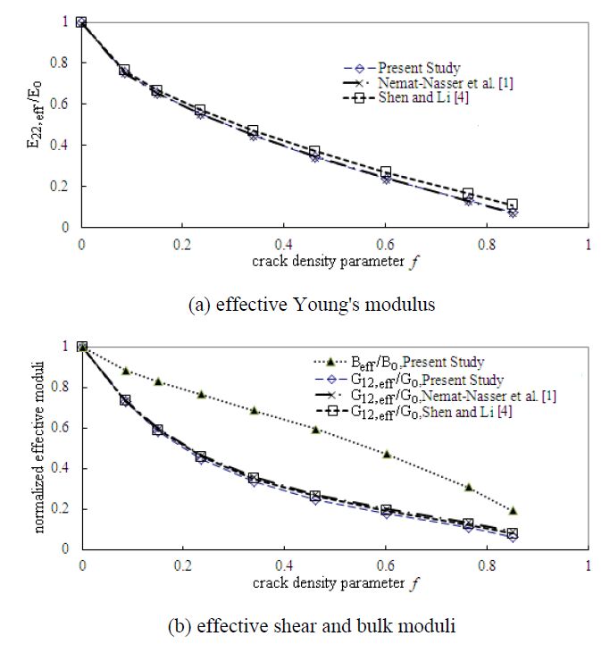
[1]	Nemat-Nasser S, Yu S, Hori M (1993) Solids with periodically distributed cracks. Int J Solids Struct 30: 2071–2095. doi: 10.1016/0020-7683(93)90052-9
[2]	Kachanov M (1992) Effective elastic properties of cracked solids: critical review of some basic concepts. Appl Mech Rev 45: 304–335. doi: 10.1115/1.3119761
[3]	Petrova V, Tamuzs V, Romalis N (2000) A survey of macro-microcrack interaction problems. Appl Mech Rev 53: 1459–1472.
[4]	Shen L, Li J (2004) A numerical simulation for effective elastic moduli of plates with various distributions and sizes of cracks. Int J Solids Struct 41: 7471–7492. doi: 10.1016/j.ijsolstr.2004.02.016
[5]	Jasiuk I (1995) Cavities vis-a-vis rigid inclusions: Elastic moduli of materials with polygonal inclusions. Int J Solids Struct 32: 407–422. doi: 10.1016/0020-7683(94)00119-H
[6]	Nozaki H, Taya M (2001) Elastic fields in a polyhedral inclusion with uniform eigenstrains and related problems. J Appl Mech 68: 441–452. doi: 10.1115/1.1362670
[7]	Tsukrov I, Novak J (2004) Effective elastic properties of solids with two-dimensional inclusions of irregular shapes. Int J Solids Struct 41: 6905–6924. doi: 10.1016/j.ijsolstr.2004.05.037
[8]	Chang JH, Liu DY (2009) Damage assesssment for 2-D multi-cracked materials/structures by using Mc-integral. ASCE J Eng Mech 135: 1100–1107. doi: 10.1061/(ASCE)0733-9399(2009)135:10(1100)
[9]	Miehe C, Schröder J, Schotte J (1999) Computational homogenization analysis in finite plasticity. Simulation of texture development in polycrystalline materials. Comput Method Appl M 171: 387–418.
[10]	Kouznetsova VG, Brekelmans WAM, Baaijens FPT (2001) An approach to micro-macro modeling of heterogeneous materials. Comput Mech 27: 37–48. doi: 10.1007/s004660000212
[11]	Mistler M, Anthoine A, Butenweg C (2007) In-plane and out-of-plane homogenisation of masonry. Comput Struct 85: 1321–1330. doi: 10.1016/j.compstruc.2006.08.087
[12]	Shabana YM, Noda N (2008) Numerical evaluation of the thermomechanical effective properties of a functionally graded material using the homogenization method. Int J Solids Struct 45: 3494–3506. doi: 10.1016/j.ijsolstr.2008.02.012
[13]	Matous K, Kulkarni MG, Geubelle PH (2008) Multiscale cohesive failure modeling of heterogeneous adhesives. J Mech Phys Solids 56: 1511–1533. doi: 10.1016/j.jmps.2007.08.005
[14]	Hirschberger CB, Ricker S, Steinmann P, et al. (2009) Computational multiscale modelling of heterogeneous material layers. Eng Fract Mech 76: 793–812. doi: 10.1016/j.engfracmech.2008.10.018
[15]	Pham NKH, Kouznetsova V, Geers MGD (2013) Transient computational homogenization for heterogeneous materials under dynamic excitation. J Mech Phys Solids 61: 2125–2146. doi: 10.1016/j.jmps.2013.07.005
[16]	Belytschko T, Xiao SP (2003) Coupling methods for continuum model with molecular model. Int J Multiscale Com 1: 115–126.
[17]	Liu WK, Park HS, Qian D, et al. (2006) Bridging scale methods for nanomechanics and materials. Comput Method Appl M 195: 1407–1421. doi: 10.1016/j.cma.2005.05.042
[18]	Budarapu PR, Gracie R, Bordas S, et al. (2014) An adaptive multiscale method for quasi-static crack growth. Comput Mech 53: 1129–1148. doi: 10.1007/s00466-013-0952-6
[19]	Budarapu PR, Gracie R, Shih WY, et al. (2014) Efficient coarse graining in multiscale modeling of fracture. Theor Appl Fract Mec 69: 126–143. doi: 10.1016/j.tafmec.2013.12.004
[20]	Talebi H, Silani M, Rabczuk T (2015) Concurrent multiscale modelling of three dimensional crack and dislocation propagation. Adv Eng Softw 80: 82–92. doi: 10.1016/j.advengsoft.2014.09.016
[21]	Yang SW, Budarapu PR, Mahapatra DR, et al. (2015) A meshless adaptive multiscale method for fracture. Comp Mater Sci 96: 382–395. doi: 10.1016/j.commatsci.2014.08.054
[22]	Eshelby JD (1957) The determination of the elastic field of an ellipsoidal inclusion and related problems. Proceedings of the Royal Society of London A: Mathematical, Physical and Engineering Sciences. The Royal Society, 241: 376–396.
[23]	Walpole LJ (1969) On the overall elastic moduli of composite materials. J Mech Phys Solids 17: 235–251. doi: 10.1016/0022-5096(69)90014-3
[24]	Kachanov M, Tsukrov I, Shafiro B (1994) Effective properties of solids with cavities of various shapes. Appl Mech Rev 47: 151–174.
[25]	Gasser TC, Ogden RW, Holzapfel GA (2006) Hyperelastic modelling of arterial layers with distributed collagen fibre orientations. J R Soc Interface 3: 15–35. doi: 10.1098/rsif.2005.0073
[26]	Ogden RW (1984) Non-Linear Elastic Deformation, Ellis Horwood Limited, England.

Reader Comments

Your name:*

Email:*
© 2016 the Author(s), licensee AIMS Press. This is an open access article distributed under the terms of the Creative Commons Attribution License (http://creativecommons.org/licenses/by/4.0)