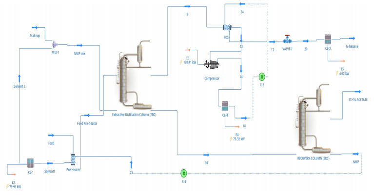
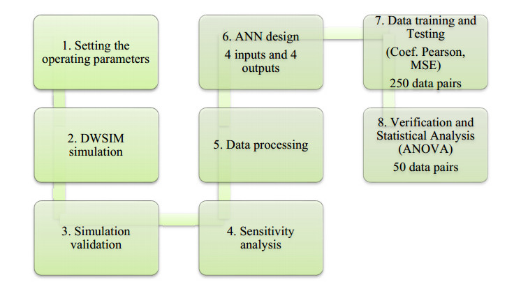
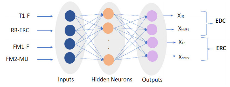
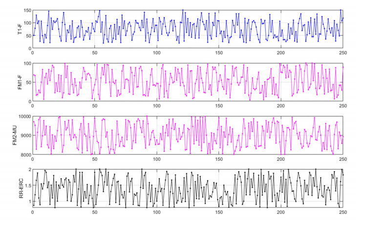
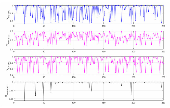
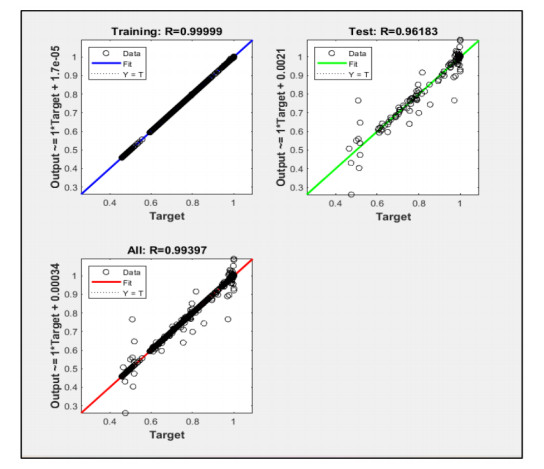
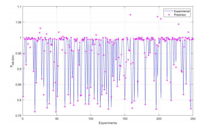
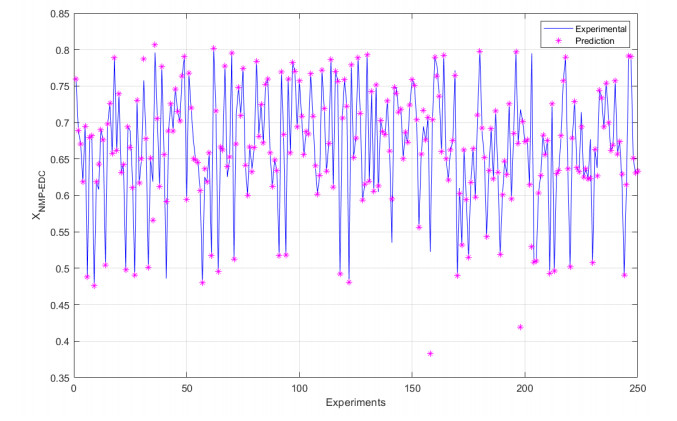
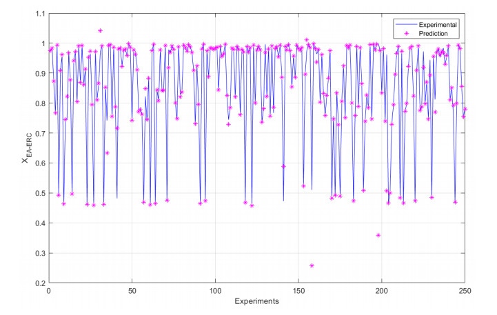
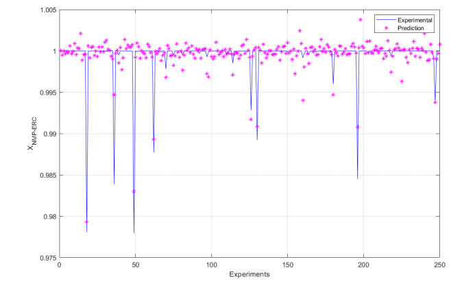
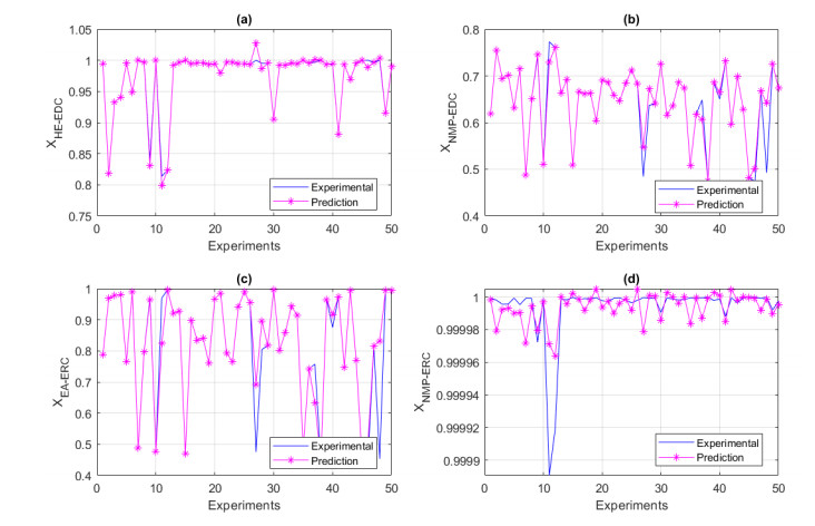
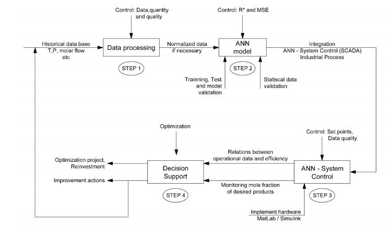
We developed an artificial neural network (ANN) to predict mole fractions in the extractive distillation of an n-hexane and ethyl acetate mixture, which are common organic solvents in chemical and pharmaceutical manufacturing. The ANN was trained on 250 data pairs from simulations in DWSIM software. The training dataset consisted of four inputs: Feed flow inlet (T1-F), Feed Stream Mass Flow temperature pressure (FM1-F), Make-up stream mass flow (FM2-MU), and ERC tower reflux ratio (RR-ERC). The ANN demonstrated the ability to forecast four output variables (neurons): Mole fraction of n-hexane in the distillate of EDC (XHE-EDC), Mole fraction of N-methyl-2 pyrrolidone in the bottom of EDC (XNMP-EDC), Mole fraction of ethyl acetate in the distillate of ERC (XEA-ERC), and Mole fraction of N-methyl-2 pyrrolidone in the bottom of ERC (XNMP-ERC).The ANN architecture contained 80 hidden neurons. Bayesian regularization training yielded high prediction accuracy (MSE = 2.56 × 10⁻⁷, R = 0.9999). ANOVA statistical validation indicated that ANN could reliably forecast mole fractions. By integrating this ANN into process control systems, manufacturers could enhance product quality, decrease operating expenses, and mitigate composition variability risks. This data-driven modeling approach may also optimize energy consumption when combined with genetic algorithms. Further research will validate predictions onsite and explore hybrid energy optimization technologies.
Citation: Daniel Chuquin-Vasco, Dennise Chicaiza-Sagal, Cristina Calderón-Tapia, Nelson Chuquin-Vasco, Juan Chuquin-Vasco, Lidia Castro-Cepeda. Forecasting mixture composition in the extractive distillation of n-hexane and ethyl acetate with n-methyl-2-pyrrolidone through ANN for a preliminary energy assessment[J]. AIMS Energy, 2024, 12(2): 439-463. doi: 10.3934/energy.2024020
We developed an artificial neural network (ANN) to predict mole fractions in the extractive distillation of an n-hexane and ethyl acetate mixture, which are common organic solvents in chemical and pharmaceutical manufacturing. The ANN was trained on 250 data pairs from simulations in DWSIM software. The training dataset consisted of four inputs: Feed flow inlet (T1-F), Feed Stream Mass Flow temperature pressure (FM1-F), Make-up stream mass flow (FM2-MU), and ERC tower reflux ratio (RR-ERC). The ANN demonstrated the ability to forecast four output variables (neurons): Mole fraction of n-hexane in the distillate of EDC (XHE-EDC), Mole fraction of N-methyl-2 pyrrolidone in the bottom of EDC (XNMP-EDC), Mole fraction of ethyl acetate in the distillate of ERC (XEA-ERC), and Mole fraction of N-methyl-2 pyrrolidone in the bottom of ERC (XNMP-ERC).The ANN architecture contained 80 hidden neurons. Bayesian regularization training yielded high prediction accuracy (MSE = 2.56 × 10⁻⁷, R = 0.9999). ANOVA statistical validation indicated that ANN could reliably forecast mole fractions. By integrating this ANN into process control systems, manufacturers could enhance product quality, decrease operating expenses, and mitigate composition variability risks. This data-driven modeling approach may also optimize energy consumption when combined with genetic algorithms. Further research will validate predictions onsite and explore hybrid energy optimization technologies.

| [1] |
Feng ZF, Shen WF, Rangaiah GP, et al. (2020) Design and control of vapor recompression assisted extractive distillation for separating n-hexane and ethyl acetate. Sep Purif Technol 240: 116655. https://doi.org/10.1016/j.seppur.2020.116655 doi: 10.1016/j.seppur.2020.116655

|
| [2] |
Acosta J, Arce A, Martı́nez-Ageitos J, et al. (2002) Vapor-Liquid equilibrium of the ternary system ethyl Acetate+ Hexane+ acetone at 101.32 kPa. J Chem Eng Data 47: 849–854. https://doi.org/10.1021/je0102917 doi: 10.1021/je0102917
|
| [3] |
Yang Kong Z, Yeh Lee H, Sunarso J (2022) The evolution of process design and control for ternary azeotropic separation: Recent advances in distillation and future directions. Sep Purif Technol 284: 120292. https://doi.org/10.1016/j.seppur.2021.120292 doi: 10.1016/j.seppur.2021.120292
|
| [4] |
Gerbaud V, Rodriguez-Donis I, Hegely L, et al. (2019) Review of extractive distillation. Process design, operation, optimization and control. Chem Eng Res Des 141: 229–271. https://doi.org/10.1016/j.cherd.2018.09.020 doi: 10.1016/j.cherd.2018.09.020
|
| [5] |
Iqbal A, Akhlaq Ahmad S, Ojasvi (2019) Design and control of an energy-efficient alternative process for separation of dichloromethane-methanol binary azeotropic mixture. Sep Purif Technol 219: 137–149. https://doi.org/10.1016/j.seppur.2019.03.005 doi: 10.1016/j.seppur.2019.03.005
|
| [6] |
Zhu Z, Yu X, Ma Y, et al. (2020) Efficient extractive distillation design for separating binary azeotrope via thermodynamic and dynamic analyses. Sep Purif Technol 238: 116425. https://doi.org/10.1016/j.seppur.2019.116425 doi: 10.1016/j.seppur.2019.116425
|
| [7] |
Yang X, Ward J (2018) Design of a pressure-swing distillation process for the separation of n-hexane and ethyl acetate using simulated annealing. Comp Aid Chem Eng 44: 121–126. https://doi.org/10.1016/B978-0-444-64241-7.50015-X doi: 10.1016/B978-0-444-64241-7.50015-X
|
| [8] |
Lü L, Zhu L, Liu H, et al. (2018) Comparison of continuous homogenous azeotropic and pressure-swing distillation for a minimum azeotropic system ethyl acetate/n-hexane separation. Chin J Chem Eng 26: 2023–2033. https://doi.org/10.1016/j.cjche.2018.02.002 doi: 10.1016/j.cjche.2018.02.002
|
| [9] |
Li Y, Sun T, Ye Q, et al. (2021) Investigation on energy-efficient extractive distillation for the recovery of ethyl acetate and 1, 4-dioxane from industrial effluent. J Clean Prod 329: 129759. https://doi.org/10.1016/j.jclepro.2021.129759 doi: 10.1016/j.jclepro.2021.129759
|
| [10] |
Shi F, Gao J, Huang X (2016) An affine invariant approach for dense wide baseline image matching. Int J Distrib Sens Netw, 12. https://doi.org/10.1177/1550147716680826 doi: 10.1177/1550147716680826
|
| [11] |
Sun L, Liang F, Cui W (2021) Artificial neural network and its application research progress in chemical process. Asian J Res Comput Sci 12: 177–185. https://doi.org/10.9734/ajrcos/2021/v12i430302 doi: 10.9734/ajrcos/2021/v12i430302
|
| [12] | Singh RP, Heldman DR (2008) Introduction to food engineering. A volume in Food science and technology, Fifth Eds., California: Academic Press. Available from: https://www.sciencedirect.com/book/9780123985309/introduction-to-food-engineering. |
| [13] |
Elgibaly A, Ghareeb M, Kamel S, et al. (2021) Prediction of gas-lift performance using neural network analysis. AIMS Energy 9: 355–378. https://doi.org/10.3934/energy.2021019 doi: 10.3934/energy.2021019
|
| [14] |
Kandil A, Khaled S, Elfakharany T (2023) Prediction of the equivalent circulation density using machine learning algorithms based on real-time data. AIMS Energy 11: 425–453. https://doi.org/10.3934/energy.2023023 doi: 10.3934/energy.2023023
|
| [15] |
Hamdi M, El Salmawy H, Ragab R (2023) Optimum configuration of a dispatchable hybrid renewable energy plant using artificial neural networks: Case study of Ras Ghareb, Egypt. AIMS Energy 11: 171–196. https://doi.org/10.3934/energy.2023010 doi: 10.3934/energy.2023010
|
| [16] |
Aly A, Saleh B, Bassuoni M, et al. (2019) Artificial neural network model for performance evaluation of an integrated desiccant air conditioning system activated by solar energy. AIMS Energy 7: 395–412. https://doi.org/10.3934/energy.2019.3.395 doi: 10.3934/energy.2019.3.395
|
| [17] |
Zhang Z, Zhao J (2017) A deep belief network based fault diagnosis model for complex chemical processes. Comput Chem Eng 107: 395–407. https://doi.org/10.1016/j.compchemeng.2017.02.041 doi: 10.1016/j.compchemeng.2017.02.041
|
| [18] |
Yazdizadeh M, Jafari Nasr M, Safekordi A (2016) A new catalyst for the production of furfural from bagasse. RSC Adv 61: 55778–55785. https://doi.org/10.1039/c6ra10499a doi: 10.1039/c6ra10499a
|
| [19] |
Esonye C, Dominic Onukwuli O, Uwaoma Ofoefule A (2019) Optimization of methyl ester production from Prunus amygdalus seed oil using response surface methodology and artificial neural networks. Renewable Energy 130: 61–72. https://doi.org/10.1016/j.renene.2018.06.036 doi: 10.1016/j.renene.2018.06.036
|
| [20] |
Ge X, Wang B, Yang X, et al. (2021) Fault detection and diagnosis for reactive distillation based on convolutional neural network. Comput Chem Eng 145: 107172. https://doi.org/10.1016/j.compchemeng.2020.107172 doi: 10.1016/j.compchemeng.2020.107172
|
| [21] |
de Araújo Neto AP, Sales FA, Brito RP (2021) Controllability comparison for extractive dividing-wall columns: ANN-based intelligent control system versus conventional control system. Chem Eng Proc Intens 160: 108271. https://doi.org/10.1016/j.cep.2020.108271 doi: 10.1016/j.cep.2020.108271
|
| [22] |
Inyang V, Lokhat D (2022) Propionic acid recovery from dilute aqueous solution by emulsion liquid membrane (ELM) technique: optimization using response surface methodology (RSM) and artificial neural network (ANN) experimental design. Sep Scie Tech 57: 284–300. https://doi.org/10.1080/01496395.2021.1890774 doi: 10.1080/01496395.2021.1890774
|
| [23] | DWSIM (2020) DWSIM—The open source chemical process simulator. Available from: https://dwsim.org. |
| [24] |
Chuquin-Vasco D, Parra F, Chuquin-Vasco N, et al. (2021) Prediction of methanol production in a carbon dioxide hydrogenation plant using neural networks. Energies 14: 1–18. https://doi.org/10.3390/en14133965 doi: 10.3390/en14133965
|
| [25] |
Dimian AC, Bildea CS, Kiss AA (2014) Introduction in process simulation. Comput Aided Chem Eng 35: 35–71. https://doi.org/10.1016/B978-0-444-62700-1.00002-4 doi: 10.1016/B978-0-444-62700-1.00002-4
|
| [26] | Kiss AA (2013) Advanced distillation technologies: Design, control and applications. 1 Eds., Noida, India: Wiley. https://doi.org/10.1002/9781118543702 |
| [27] |
Soave G, Gamba S, Pellegrini L (2010) SRK equation of state: predicting binary interaction parameters of hydrocarbons and related compounds. Fluid Phase 299: 285–293. https://doi.org/10.1016/j.fluid.2010.09.012 doi: 10.1016/j.fluid.2010.09.012
|
| [28] |
Hu Y, Wang J, Tan C, et al. (2017) Further improvement of fluidized bed models by incorporating zone method with Aspen Plus interface. Energy Proc 105: 1895–1901. https://doi.org/10.1016/j.egypro.2017.03.556 doi: 10.1016/j.egypro.2017.03.556
|
| [29] |
Mlazi NJ, Mayengo M, Lyakurwa G, et al. (2024) Mathematical modeling and extraction of parameters of solar photovoltaic module based on modified Newton-Raphson method. Results Phys 57: 107364. https://doi.org/10.1016/j.rinp.2024.107364 doi: 10.1016/j.rinp.2024.107364
|
| [30] |
Chen Y, Song L, Liu Y, et al. (2020) A review of the artificial neural network models for water quality prediction. Appl Sci 10: 5776. https://doi.org/10.3390/app10175776 doi: 10.3390/app10175776
|
| [31] |
Singh V, Gupta I, Gupta H (2005) ANN based estimator for distillation-inferential control. Chem Eng Proc Int 44: 785–795. https://doi.org/10.1016/j.cep.2004.08.010 doi: 10.1016/j.cep.2004.08.010
|
| [32] | Pedregosa F, Varaquaux G, Gramfort A, et al. (2011) Scikit-learn: machine learning in Python. J Mach Lear Res. Available from: https://www.jmlr.org/papers/volume12/pedregosa11a/pedregosa11a.pdf. |
| [33] |
Bloice M, Holzinger A (2016) A tutorial on machine learning and data science tools with python. Lect Not Comp Sci 9605: 435–480. https://doi.org/10.1007/978-3-319-50478-0_22 doi: 10.1007/978-3-319-50478-0_22
|
| [34] |
Purna Pushkala S, Panda R (2023) Design and analysis of reactive distillation for the production of isopropyl myristate. Clean Chem Eng 5: 100090. https://doi.org/10.1016/j.clce.2022.100090 doi: 10.1016/j.clce.2022.100090
|
| [35] |
Elsheikh M, Ortmanns Y, Hecht F, et al. (2023) Control of an industrial distillation column using a hybrid model with adaptation of the range of validity and an ANN-based soft sensor. Chem Ing Tech 95: 1114–1124. https://doi.org/10.1002/cite.202200232 doi: 10.1002/cite.202200232
|
| [36] |
Neves T, De Araújo Neto A, Sales F, et al. (2021) ANN-based intelligent control system for simultaneous feed disturbances rejection and product specification changes in extractive distillation process. Sep Purif Technol 259: 118404. https://doi.org/10.1016/j.seppur.2020.118104 doi: 10.1016/j.seppur.2020.118104
|
| [37] |
Kayri M (2016) Predictive abilities of bayesian regularization and levenberg-marquardt algorithms in artificial neural networks: A comparative empirical study on social data. Math Comp App 21: 20. https://doi.org/10.3390/mca21020020 doi: 10.3390/mca21020020
|
| [38] |
Bharati S, Atikur Rahman M, Podder P, et al. (2021) Comparative performance analysis of neural network base training algorithm and neuro-fuzzy system with SOM for the purpose of prediction of the features of superconductors. Int Syst Des App 1181: 69–79. https://doi.org/10.1007/978-3-030-49342-4_7 doi: 10.1007/978-3-030-49342-4_7
|
| [39] |
Mohan Saini L (2008) Peak load forecasting using bayesian regularization, resilient and adaptive backpropagation learning based artificial neural networks. Elec Power Syst Res 78: 1302–1310. https://doi.org/10.1016/j.epsr.2007.11.003 doi: 10.1016/j.epsr.2007.11.003
|
| [40] |
Wang L, Wu B, Zhu Q, et al. (2020) Forecasting monthly tourism demand using enhanced backpropagation neural network. Neural Process Lett 52: 2607–2636. https://doi.org/10.1007/s11063-020-10363-z doi: 10.1007/s11063-020-10363-z
|
| [41] |
Zeng Y, Zeng Y, Choi B, et al. (2017) Multifactor-influenced energy consumption forecasting using enhanced back-propagation neural network. Energy 127: 381–396. https://doi.org/10.1016/j.energy.2017.03.094 doi: 10.1016/j.energy.2017.03.094
|
| [42] |
Suphawan K, Chaisee K (2021) Gaussian process regression for predicting water quality index: A case study on ping river basin, thailand. AIMS Environ Sci 8: 268–282. https://doi.org/10.3934/environsci.2021018 doi: 10.3934/environsci.2021018
|
| [43] |
Wang L, Wu B, Zhu Q, et al. (2020) Forecasting monthly tourism demand using enhanced backpropagation neural network. Neural Process Lett 52: 2607–2636. https://doi.org/10.1007/s11063-020-10363-z doi: 10.1007/s11063-020-10363-z
|
| [44] |
Zhang L, Sun X, Gao S (2022) Temperature prediction and analysis based on improved GA-BP neural network. AIMS Environ Sci 9: 735–753. https://doi.org/10.3934/environsci.2022042 doi: 10.3934/environsci.2022042
|
| [45] |
Suliman A, Omarov B (2018) Applying bayesian regularization for acceleration of levenberg marquardt based neural network training. Int J Int Mult Art Inte 5: 68. https://doi.org/10.9781/ijimai.2018.04.004 doi: 10.9781/ijimai.2018.04.004
|
| [46] |
Garoosiha H, Ahmadi J, Bayat H (2019) The assessment of Levenberg-marquardt and bayesian Framework training algorithm for prediction of concrete shrinkage by the artificial neural network. Cogent Eng 6: 1609179. https://doi.org/10.1080/23311916.2019.1609179 doi: 10.1080/23311916.2019.1609179
|
| [47] |
Kim R, Min J, Lee J, et al. (2023) Development of bayesian regularized artificial neural network for airborne chlorides estimation. Constr Build Mater 383: 131361. https://doi.org/10.1016/j.conbuildmat.2023.131361 doi: 10.1016/j.conbuildmat.2023.131361
|
| [48] |
Yalamanchi K, Kommalapati S, Pal P, et al. (2023) Uncertainty quantification of a deep learning fuel property prediction model. Appl Energy Comb Sci 16: 100211. https://doi.org/10.1016/j.jaecs.2023.100211 doi: 10.1016/j.jaecs.2023.100211
|
| [49] |
Jog S, Vázquez D, Santos L, et al. (2023) Hybrid analytical surrogate-based process optimization via bayesian symbolic regression. Comput Chem Eng 182: 108563. https://doi.org/10.1016/j.compchemeng.2023.108563 doi: 10.1016/j.compchemeng.2023.108563
|
| [50] |
Abiodun O, Jantan A, Omolara A, et al. (2018) State of the art in artificial neural network applications: A survey. Heliyon 4: E00938. https://doi.org/10.1016/j.heliyon.2018.e00938 doi: 10.1016/j.heliyon.2018.e00938
|
| [51] | Tgarguifa A, Bounahmidi T, Fellaou S (2020) Optimal design of the distillation process using the artificial neural networks method. 2020 1st International Conference on Innovative Research in Applied Science, Engineering and Technology (IRASET), Meknes, Morocco, 1–6. Available from: https://ieeexplore.ieee.org/document/9092266. |
| [52] |
Kyono K, Hashimoto T, Nagai Y, et al. (2018) Analysis of endometrial microbiota by 16S ribosomal RNA gene sequencing among infertile patients: a single-center pilot study. Reprod Med Biol 17: 297–306. https://doi.org/10.1002/rmb2.12105 doi: 10.1002/rmb2.12105
|
| [53] |
Talaei Khoei T, Ould Slimane H, Kaabouch N (2023) Deep learning: Systematic review, models, challenges, and research directions. Neural Comput Appl 35: 23103–23124. https://doi.org/10.1007/s00521-023-08957-4 doi: 10.1007/s00521-023-08957-4
|
| [54] |
Boger Z (1997) Experience in industrial plant model development using large-scale artificial neural networks. Inf Sci 101: 203–216. https://doi.org/10.1016/S0020-0255(97)00010-8 doi: 10.1016/S0020-0255(97)00010-8
|
| [55] |
Acevedo L, Uche J, Del-Amo A (2018) Improving the distillate prediction of a membrane distillation unit in a trigeneration scheme by using artificial neural networks. Water 10: 310. https://doi.org/10.3390/w10030310 doi: 10.3390/w10030310
|
| [56] |
Shin Y, Smith R, Hwang S (2020) Development of model predictive control system using an artificial neural network: A case study with a distillation column. J Clean Prod 277: 124124. https://doi.org/10.1016/j.jclepro.2020.124124 doi: 10.1016/j.jclepro.2020.124124
|
| [57] |
Magdy Saady M, Hassan Essai M (2022) Hardware implementation of neural network-based engine model using FPGA. Alex Eng J 61: 12039–12050. https://doi.org/10.1016/j.aej.2022.05.035 doi: 10.1016/j.aej.2022.05.035
|
| [58] |
Hasimi L, Zavantis D, Shakshuki E, et al. (2024) Cloud computing security and deep learning: An ANN approach. Proc Comp Sci 231: 40–47. https://doi.org/10.1016/j.procs.2023.12.155 doi: 10.1016/j.procs.2023.12.155
|
 energy-12-02-020 Supplementary.pdf energy-12-02-020 Supplementary.pdf |
 |

Figures(13) / Tables(12)

Daniel Chuquin-Vasco, Dennise Chicaiza-Sagal, Cristina Calderón-Tapia, Nelson Chuquin-Vasco, Juan Chuquin-Vasco, Lidia Castro-Cepeda. Forecasting mixture composition in the extractive distillation of n-hexane and ethyl acetate with n-methyl-2-pyrrolidone through ANN for a preliminary energy assessment[J]. AIMS Energy, 2024, 12(2): 439-463. doi: 10.3934/energy.2024020


 DownLoad: