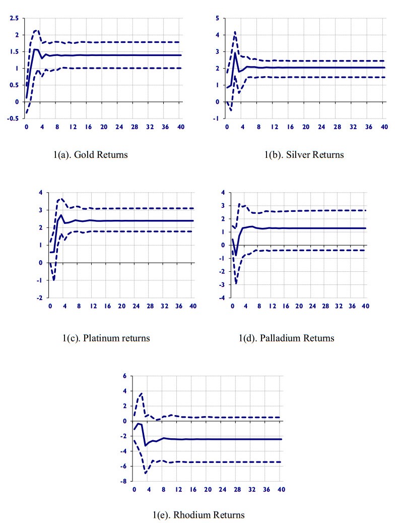
We examine the potential of gold and other precious metals as safe havens during negative market shocks caused by the Global Financial Cycle (GFCy). We analyze a vast global vector autoregressive (GVAR) model that includes developing and emerging market countries for a total of 33 countries, from 1979:Q2 to 2019:Q4. This approach allows us to account for individual country peculiarities while also considering the transmission of global shocks. We found that during financial market distress caused by a negative GFCy shock, gold, silver and platinum all serve as hedges. Interestingly, our results suggest that silver and platinum are better hedges than gold, offering greater positive returns in response to negative GFCy shocks, especially in recent years. Overall, our findings support the benefits of investing in precious metals, as they can help investors mitigate losses resulting from global financial shocks. While the metals vary in their hedging ability, platinum and silver offer even greater protection than gold.
Citation: Afees A. Salisu, Rangan Gupta, Siphesihle Ntyikwe, Riza Demirer. Gold and the global financial cycle[J]. Quantitative Finance and Economics, 2023, 7(3): 475-490. doi: 10.3934/QFE.2023024
We examine the potential of gold and other precious metals as safe havens during negative market shocks caused by the Global Financial Cycle (GFCy). We analyze a vast global vector autoregressive (GVAR) model that includes developing and emerging market countries for a total of 33 countries, from 1979:Q2 to 2019:Q4. This approach allows us to account for individual country peculiarities while also considering the transmission of global shocks. We found that during financial market distress caused by a negative GFCy shock, gold, silver and platinum all serve as hedges. Interestingly, our results suggest that silver and platinum are better hedges than gold, offering greater positive returns in response to negative GFCy shocks, especially in recent years. Overall, our findings support the benefits of investing in precious metals, as they can help investors mitigate losses resulting from global financial shocks. While the metals vary in their hedging ability, platinum and silver offer even greater protection than gold.

| [1] |
Adekoya OB, Oliyide JA (2021) How COVID-19 drives connectedness among commodity and financial markets: Evidence from TVP-VAR and causality-in-quantiles techniques. Resour Policy 70: 101898. https://doi.org/10.1016/j.resourpol.2020.101898 doi: 10.1016/j.resourpol.2020.101898

|
| [2] |
Agyei-Ampomah S, Gounopoulos D, Mazouz K (2014) Does gold offer a better protection against sovereign debt crisis than other metals? J Bank Financ 40: 507–521. https://doi.org/10.1016/j.jbankfin.2013.11.014 doi: 10.1016/j.jbankfin.2013.11.014
|
| [3] |
Alonso E, Field FR, Kirchain RE (2012) Platinum Availability for Future Automotive Technologies. Environ Sci Technol 46: 12986–12993. https://doi.org/10.1021/es301110e doi: 10.1021/es301110e
|
| [4] |
Aye GC, Carcel H, Gil-Alana LA, et al. (2017) Does gold act as a hedge against inflation in the UK? Evidence from a fractional cointegration approach over 1257 to 2016. Resour Pol 54: 53–57. https://doi.org/10.1016/j.resourpol.2017.09.001 doi: 10.1016/j.resourpol.2017.09.001
|
| [5] |
Aye GC, Chang T, Gupta R (2016) Is gold an inflation-hedge? Evidence from an interrupted Markov-switching co-integration model. Resour Policy 44: 77–84. https://doi.org/10.1016/j.resourpol.2016.02.011 doi: 10.1016/j.resourpol.2016.02.011
|
| [6] |
Aye GC, Gupta R, Hammoudeh S, et al. (2015) Forecasting the price of gold using dynamic model averaging. Int Rev Financ Anal 41: 257–266. https://doi.org/10.1016/j.irfa.2015.03.010 doi: 10.1016/j.irfa.2015.03.010
|
| [7] |
Balcilar M, Bonato M, Demirer R, et al. (2017) The effect of investor sentiment on gold market return dynamics: Evidence from a nonparametric causality-in-quantiles approach. Resour Pol 51: 77–84. https://doi.org/10.1016/j.resourpol.2016.11.009 doi: 10.1016/j.resourpol.2016.11.009
|
| [8] |
Balcilar M, Demirer R, Gupta R, et al. (2020) The effect of global and regional stock market shocks on safe haven assets. Structur Change Econ D 54: 297–308. https://doi.org/10.1016/j.strueco.2020.04.004 doi: 10.1016/j.strueco.2020.04.004
|
| [9] |
Balcilar M, Gupta R, Nguyen DK, et al. (2018) Causal effects of the United States and Japan on Pacific-Rim stock markets: nonparametric quantile causality approach. Appl Econ 50: 5712–5727. https://doi.org/10.1080/00036846.2018.1488062 doi: 10.1080/00036846.2018.1488062
|
| [10] |
Balcilar M, Gupta R, Pierdzioch C (2016) Does uncertainty move the gold price? New evidence from a nonparametric causality-in-quantiles test. Resour Policy 49: 74–80. https://doi.org/10.1016/j.resourpol.2016.04.004 doi: 10.1016/j.resourpol.2016.04.004
|
| [11] |
Bampinas G, Panagiotidis T (2015) Are gold and silver a hedge against inflation? A two century perspective. Int Rev Financ Anal 41: 267–276. https://doi.org/10.1016/j.irfa.2015.02.007 doi: 10.1016/j.irfa.2015.02.007
|
| [12] |
Baur DG, Lucey BM (2010) Is gold a hedge or a safe haven? An analysis of stocks, bonds and gold. Financ Rev 45: 217–229. https://doi.org/10.1111/j.1540-6288.2010.00244.x doi: 10.1111/j.1540-6288.2010.00244.x
|
| [13] |
Baur DG, McDermott TK (2010) Is gold a safe haven? International evidence. J Bank Financ 34: 1886–1898. https://doi.org/10.1016/j.jbankfin.2009.12.008 doi: 10.1016/j.jbankfin.2009.12.008
|
| [14] |
Baur, D.G., Smales, L.A. (2020) Hedging geopolitical risk with precious metals. J Bank Financ 117: 105823. https://doi.org/10.1016/j.jbankfin.2020.105823 doi: 10.1016/j.jbankfin.2020.105823
|
| [15] |
Beaino G, Lombardi D, Siklos PL (2018) The Transmission of Financial Shocks on a Global Scale: Some New Empirical Evidence. Emerg Mark Financ Tr 55: 1634–1655. https://doi.org/10.1080/1540496X.2018.1481046 doi: 10.1080/1540496X.2018.1481046
|
| [16] |
Beckmann J, Berger T, Czudaj R (2015) Does gold act a hedge or safe haven for stocks? A smooth transition approach. Econ Model 48: 16–24. https://doi.org/10.1016/j.econmod.2014.10.044 doi: 10.1016/j.econmod.2014.10.044
|
| [17] |
Beckmann J, Berger T, Czudaj R (2019) Gold Price Dynamics and the Role of Uncertainty. Quant Financ 19: 663–681. https://doi.org/10.1080/14697688.2018.1508879 doi: 10.1080/14697688.2018.1508879
|
| [18] |
Beckmann J, Czudaj R (2013) Gold as an inflation hedge in a time-varying coefficient Framework. N Am J Econ Financ 24: 208–222. https://doi.org/10.1016/j.najef.2012.10.007 doi: 10.1016/j.najef.2012.10.007
|
| [19] |
Bettendorf T (2017) Investigating Global Imbalances: Empirical evidence from a GVAR approach. Econ Model 64: 201–210. https://doi.org/10.1016/j.econmod.2017.03.033 doi: 10.1016/j.econmod.2017.03.033
|
| [20] |
Bonato M, Demirer R, Gupta R, et al. (2018) Gold futures returns and realized moments: A forecasting experiment using a quantile-boosting approach. Resour Policy 57: 196–212. https://doi.org/10.1016/j.resourpol.2018.03.004 doi: 10.1016/j.resourpol.2018.03.004
|
| [21] |
Boubaker H, Cunado J, Gil-Alana LA, et al. (2020) Global crises and gold as a safe haven: Evidence from over seven and a half centuries of data. Phys A 540: 123093. https://doi.org/10.1016/j.physa.2019.123093 doi: 10.1016/j.physa.2019.123093
|
| [22] |
Bouoiyour J, Selmi R, Wohar ME (2018) Measuring the response of gold prices to uncertainty: An analysis beyond the mean. Econ Model 75: 105–116. https://doi.org/10.1016/j.econmod.2018.06.010 doi: 10.1016/j.econmod.2018.06.010
|
| [23] |
Bouri E, Cepni O, Gabauer D, Gupta R (2021) Return connectedness across asset classes around the COVID-19 outbreak? Int Rev Financ Anal 73: 101646. https://doi.org/10.1016/j.irfa.2020.101646 doi: 10.1016/j.irfa.2020.101646
|
| [24] |
Burdekin RCK, Tao R (2021) The golden hedge: From global financial crisis to global pandemic. Econ Mod 95: 170–180. https://doi.org/10.1016/j.econmod.2020.12.009 doi: 10.1016/j.econmod.2020.12.009
|
| [25] |
Carpantier JF (2021) Anything but gold - The golden constant revisited. J Commod Mark 24: 100170. https://doi.org/10.1016/j.jcomm.2021.100170 doi: 10.1016/j.jcomm.2021.100170
|
| [26] |
Cashin P, Mohaddes K, Raissi M (2017) Fair weather or foul? The macroeconomic effects of El Niño. J Int Econ 106: 37–54. https://doi.org/10.1016/j.jinteco.2017.01.010 doi: 10.1016/j.jinteco.2017.01.010
|
| [27] |
Chudik A, Pesaran MH (2013) Econometric analysis of high dimensional VARs featuring a dominant unit. Economet Rev 32: 592–649. https://doi.org/10.1080/07474938.2012.740374 doi: 10.1080/07474938.2012.740374
|
| [28] |
Chudik A, Pesaran MH (2016) Theory and practice of GVAR modelling. J Econ Surv 30: 165–197. https://doi.org/10.1111/joes.12095 doi: 10.1111/joes.12095
|
| [29] |
Chudik A, Mohaddes K, Pesaran MH, et al. (2021) A counterfactual economic analysis of Covid-19 using a threshold augmented multi-country model. J Int Mon Fin 119: 102477. https://doi.org/10.1016/j.jimonfin.2021.102477 doi: 10.1016/j.jimonfin.2021.102477
|
| [30] | Das D, Kannadhasan M, Bhowmik P (2019) Geopolitical risk and precious metals. J Econ Res 24: 49–66. |
| [31] |
De Waal A, van Eyden R (2016) The Impact of Economic Shocks in the Rest of the World on South Africa: Evidence from a Global VAR. Emerg Mark Financ Tr 52: 557–573. https://doi.org/10.1080/1540496X.2015.1103141 doi: 10.1080/1540496X.2015.1103141
|
| [32] |
Dees S, Mauro FD, Pesaran MH, et al. (2007) Exploring the international linkages of the euro area: a global VAR analysis. J Appl Economet 22: 1–38. https://doi.org/10.1002/jae.932 doi: 10.1002/jae.932
|
| [33] |
Eickmeier S, Ng T (2015) How do US credit supply shocks propagate internationally? A GVAR approach. Eur Econ Rev 74: 128–145. https://doi.org/10.1016/j.euroecorev.2014.11.011 doi: 10.1016/j.euroecorev.2014.11.011
|
| [34] |
Feldkircher M, Huber F (2016) The International Transmission of U.S. Shocks—Evidence from Bayesian Global Vector Autoregressions. Eur Econ Rev 81: 167–188. https://doi.org/10.1016/j.euroecorev.2015.01.009 doi: 10.1016/j.euroecorev.2015.01.009
|
| [35] |
Gupta R, Majumdar A, Pierdzioch C, et al. (2017) Do terror attacks predict gold returns? Evidence from a quantile-predictive-regression approach. Q Rev Econ Financ 65: 276–284. https://doi.org/10.1016/j.qref.2017.01.005 doi: 10.1016/j.qref.2017.01.005
|
| [36] |
Gürgün G, Ünalmis I (2014) Is gold a safe haven against equity market investment in emerging and developing countries? Financ Res Lett 11: 341–348. https://doi.org/10.1016/j.frl.2014.07.003 doi: 10.1016/j.frl.2014.07.003
|
| [37] |
Hammoudeh S, Yuan Y (2008) Metal volatility in presence of oil and interest rate shocks. Energy Econ 30: 606–620. https://doi.org/10.1016/j.eneco.2007.09.004 doi: 10.1016/j.eneco.2007.09.004
|
| [38] |
Hood M, Malik F (2013) Is gold the best hedge and a safe haven under changing stock market volatility? Rev Financ Econ 22: 47–52. https://doi.org/10.1016/j.rfe.2013.03.001 doi: 10.1016/j.rfe.2013.03.001
|
| [39] |
Huang D, Kilic M (2019) Gold, platinum, and expected stock returns. J Financ Econ 132: 50–75. https://doi.org/10.1016/j.jfineco.2018.11.004 doi: 10.1016/j.jfineco.2018.11.004
|
| [40] |
Huynh TLD (2020) The effect of uncertainty on the precious metals market: New insights from Transfer Entropy and Neural Network VAR. Resour Policy 66: 101623. https://doi.org/10.1016/j.resourpol.2020.101623 doi: 10.1016/j.resourpol.2020.101623
|
| [41] |
Kempa B, Khan NS (2019) Global Macroeconomic Repercussions of US Trade Restrictions: Evidence from a GVAR Model. Int Econ J 33: 649–661. https://doi.org/10.1080/10168737.2019.1657476 doi: 10.1080/10168737.2019.1657476
|
| [42] |
Klein T (2017) Dynamic correlation of precious metals and flight-to-quality in developed markets. Fin Res Lett 23: 283–290. https://doi.org/10.1016/j.frl.2017.05.002 doi: 10.1016/j.frl.2017.05.002
|
| [43] |
Liu H, Tang X, Zhou G (2022) Recovering the FOMC risk premium. J Financ Econ 145: 45–68. https://doi.org/10.1016/j.jfineco.2022.04.005 doi: 10.1016/j.jfineco.2022.04.005
|
| [44] |
Low RKY, Yao Y, Faff R (2016) Diamonds vs. precious metals: What shines brightest in your investment portfolio? Int Rev Financ Anal 43: 1–14. https://doi.org/10.1016/j.irfa.2015.11.002 doi: 10.1016/j.irfa.2015.11.002
|
| [45] |
Lucey BM, Li S (2015) What precious metals act as safe havens, and when? Some US evidence. Appl Econ Lett 22: 35–45. https://doi.org/10.1080/13504851.2014.920471 doi: 10.1080/13504851.2014.920471
|
| [46] |
Massari S, Ruberti M (2013) Rare earth elements as critical raw materials: Focus on international markets and future strategies. Resour Pol 38: 36–43. https://doi.org/10.1016/j.resourpol.2012.07.001 doi: 10.1016/j.resourpol.2012.07.001
|
| [47] | Miranda-Agrippino S, Nenova T, Rey H (2020) Global Footprints of Monetary Policy. Discussion Papers 2004, Centre for Macroeconomics (CFM). |
| [48] |
Miranda-Agrippino S, Rey H (2020) US Monetary Policy and the Global Financial Cycle. Rev of Econ Stud 87: 2754–2776. https://doi.org/10.1093/restud/rdaa019 doi: 10.1093/restud/rdaa019
|
| [49] | Mohaddes K, Raissi M (2020) Compilation, Revision and Updating of the Global VAR (GVAR) Database, 1979Q2–2019Q4, University of Cambridge: Judge Business School (mimeo). |
| [50] |
Nier E, Sedik TS, Mondino T (2014) Gross Private Capital Flows to Emerging Markets: Can the Global Financial Cycle Be Tamed? IMF Working Paper: WP/14/196. https://doi.org/10.5089/9781498351867.001 doi: 10.5089/9781498351867.001
|
| [51] |
Ong SL, Sato K (2018) Regional or global shock? A global VAR analysis of Asian economic and financial integration. N Am J Econ Financ 46: 232–248. https://doi.org/10.1016/j.najef.2018.04.009 doi: 10.1016/j.najef.2018.04.009
|
| [52] |
Passari E, Rey H (2015) Financial flows and the international monetary system. Econ J 125: 675–698. https://doi.org/10.1111/ecoj.12268 doi: 10.1111/ecoj.12268
|
| [53] |
Pesaran MH, Schuermann T, Weiner SM (2004). Modeling Regional Interdependencies Using a Global Error-Correcting Macroeconometric Model. J Bus Econ Stat 22: 129–162. https://doi.org/10.1198/073500104000000019 doi: 10.1198/073500104000000019
|
| [54] |
Pierdzioch C, Risse M (2020) Forecasting precious metal returns with multivariate random forests. Empir Econ 58: 1167–1184. https://doi.org/10.1007/s00181-018-1558-9 doi: 10.1007/s00181-018-1558-9
|
| [55] |
Pierdzioch C, Risse M, Rohloff S (2015a) A real-time quantile-regression approach to forecasting gold returns under asymmetric loss. Resour Policy 45: 299–306. https://doi.org/10.1016/j.resourpol.2015.07.002 doi: 10.1016/j.resourpol.2015.07.002
|
| [56] |
Pierdzioch C, Risse M, Rohloff S (2015b) Forecasting gold-price fluctuations: a real-time boosting approach. Appl Econ Lett 22: 46–50. https://doi.org/10.1080/13504851.2014.925040 doi: 10.1080/13504851.2014.925040
|
| [57] |
Pierdzioch C, Risse M, Rohloff S (2014a) On the efficiency of the gold market: Results of a real-time forecasting approach. Int Rev Financ Anal 32: 95–108. https://doi.org/10.1016/j.irfa.2014.01.012 doi: 10.1016/j.irfa.2014.01.012
|
| [58] |
Pierdzioch C, Risse M, Rohloff S (2014b) The international business cycle and gold-price fluctuations. Q Rev Econ Financ 54: 292–305. https://doi.org/10.1016/j.qref.2014.01.002 doi: 10.1016/j.qref.2014.01.002
|
| [59] |
Reboredo JC (2013a) Is gold a safe haven or a hedge for the US dollar? Implications for risk management. J Bank Financ 37: 2665–2676. https://doi.org/10.1016/j.jbankfin.2013.03.020 doi: 10.1016/j.jbankfin.2013.03.020
|
| [60] |
Reboredo JC (2013b) Is gold a hedge or safe haven against oil price movements? Resour Policy 38: 130–137. https://doi.org/10.1016/j.resourpol.2013.02.003 doi: 10.1016/j.resourpol.2013.02.003
|
| [61] | Rey H (2018) Dilemma not trilemma: The global financial cycle and monetary policy independence. NBER Working Paper: 21162. |
| [62] |
Salisu AA, Ndako UB, Oloko TF (2019) Assessing the inflation hedging of gold and palladium in OECD countries. Resour Policy 62: 357–377. https://doi.org/10.1016/j.resourpol.2019.05.001 doi: 10.1016/j.resourpol.2019.05.001
|
| [63] | Sikiru AA, Salisu AA (2021) A Global VAR Analysis of Global and Regional Shock Spillovers to West African Countries. Singap Econ Rev [In press]. https://doi.org/10.1142/S0217590821410034 |
| [64] |
Stock JH, Watson MW (2003) Forecasting Output and Inflation: The Role of Asset Prices. J Econ Lit 41: 788–829. https://doi.org/10.1257/jel.41.3.788 doi: 10.1257/jel.41.3.788
|
| [65] |
Tiwari AK, Aye GC, Gupta R, et al. (2020) Gold-Oil Dependence Dynamics and the Role of Geopolitical Risks: Evidence from a Markov-Switching Time-Varying Copula Model. Energ Econ 88: 104748. https://doi.org/10.1016/j.eneco.2020.104748 doi: 10.1016/j.eneco.2020.104748
|
| [66] |
Tiwari AK, Boachie MK, Suleman MT, et al. (2021) Structure dependence between oil and agricultural commodities returns: The role of geopolitical risks. Energy 219: 119584. https://doi.org/10.1016/j.energy.2020.119584 doi: 10.1016/j.energy.2020.119584
|
| [67] |
Trung NB (2019) The spillover effects of US economic policy uncertainty on the global economy: A Global VAR approach. N Am J Econ Financ 48: 90–110. https://doi.org/10.1016/j.najef.2019.01.017 doi: 10.1016/j.najef.2019.01.017
|
| [68] |
von Arnim R, Tröster B, Staritz C, et al. (2018) Commodity price shocks and the distribution of income in commodity-dependent least-developed countries. J Polic Model 40: 434–451. https://doi.org/10.1016/j.jpolmod.2018.02.008 doi: 10.1016/j.jpolmod.2018.02.008
|
| [69] |
Wei H, Lahiri R (2019) The Impact of Commodity Price Shocks in the Presence of a Trading Relationship: A GVAR Analysis of the NAFTA. Energ Econ 80: 553–569. https://doi.org/10.1016/j.eneco.2019.01.022 doi: 10.1016/j.eneco.2019.01.022
|
 QFE-07-03-024-s001.pdf QFE-07-03-024-s001.pdf |
 |
Figures(2) / Tables(1)

Afees A. Salisu, Rangan Gupta, Siphesihle Ntyikwe, Riza Demirer. Gold and the global financial cycle[J]. Quantitative Finance and Economics, 2023, 7(3): 475-490. doi: 10.3934/QFE.2023024


 DownLoad: