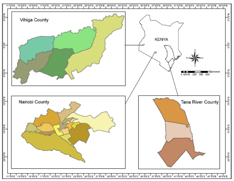
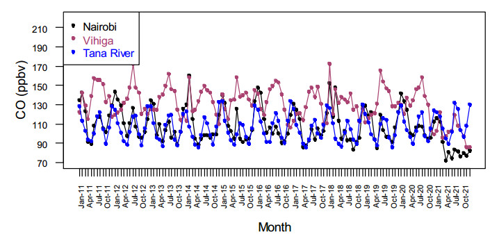
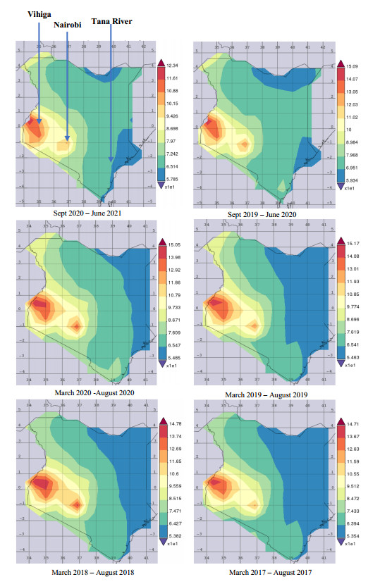
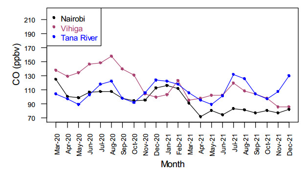
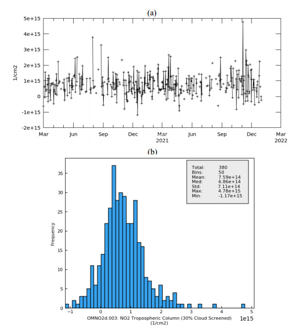
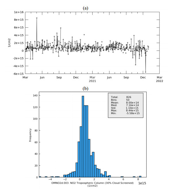
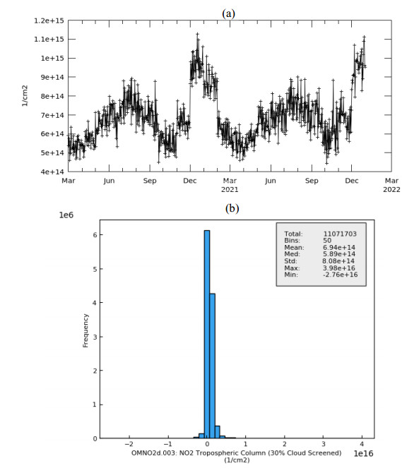
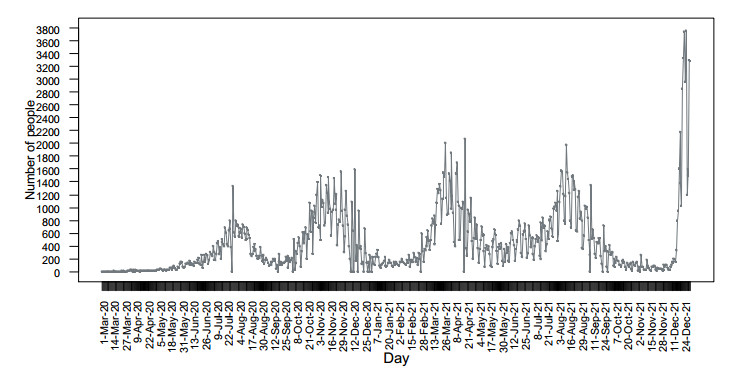
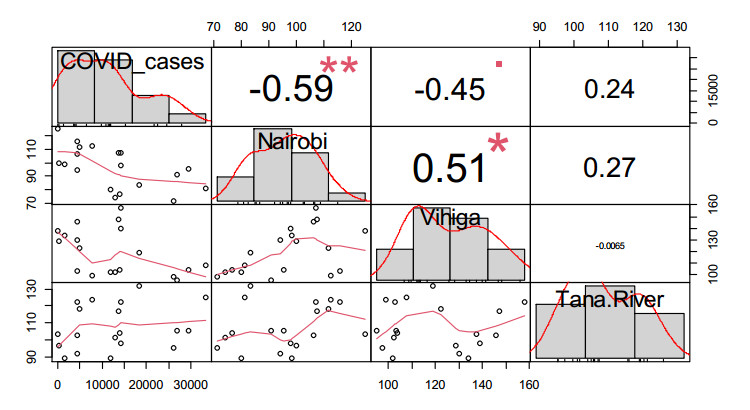
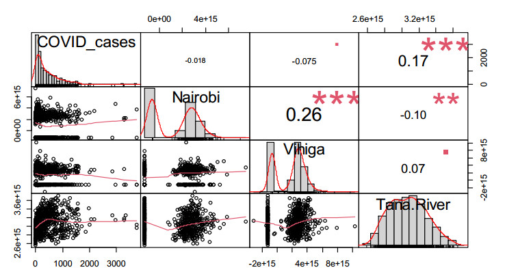
Environmental degradation, including air quality deterioration, has been mainly attributed to anthropogenic activities. Air pollution has become a pressing issue in industrialised and highly populated areas due to the combustion of fossil fuels and industrial operations. Recently, the COVID-19 pandemic led to a nationwide lockdown to control the spread of the coronavirus. This imposed restrictions on many economic activities, thus providing the environment with an opportunity to heal. The COVID-19 response measures adopted by most countries, including lockdown, restricted movement, and other containment measures, led to a significant decrease in energy use in the transport sector. Due to low electricity access levels in developing countries, traditional energy sources make up the bulk of energy used for most domestic energy services. Biomass combustion emits carbon monoxide (CO), while the transport sector is a major contributor of nitrogen dioxide (NO2). This study was purposed to investigate the short-term effects of COVID-19 on CO and NO2 concentration levels in Nairobi, Vihiga and Tana River counties. The study utilised data on CO surface concentration, NO2 column concentration and reported COVID-19 cases. Time series, correlation analysis and spatial and temporal map analysis were carried out to investigate the changes and relationships among the study parameters. The three counties were selected based on the urbanisation and population. Nairobi county represented an urban setting, while the Vihiga and Tana River counties represented rural areas with high and low population densities, respectively. The CO surface concentrations in Nairobi and Vihiga county significantly correlated with the COVID-19 cases, with both counties portraying negative correlations, i.e., −0.59 (P-value: 0.008) and −0.45 (P-value: 0.05), respectively. NO2 column concentration also exhibited a significant negative relationship with reported COVID-19 cases in the Vihiga (−0.018, P-value = 0.05) and Tana River (0.17, P-value = 0.00) counties. These findings highlight the need for demographic and economic considerations in CO and NO2 assessments, and allude to a decreased health risk due to CO and NO2 emissions during the COVID-19 pandemic.
Citation: Cohen Ang'u, Nzioka John Muthama, Mwanthi Alexander Mutuku, Mutembei Henry M'IKiugu. Carbon monoxide and nitrogen dioxide patterns associated with changes in energy use during the COVID-19 pandemic in Kenya[J]. AIMS Environmental Science, 2022, 9(3): 244-259. doi: 10.3934/environsci.2022017
Environmental degradation, including air quality deterioration, has been mainly attributed to anthropogenic activities. Air pollution has become a pressing issue in industrialised and highly populated areas due to the combustion of fossil fuels and industrial operations. Recently, the COVID-19 pandemic led to a nationwide lockdown to control the spread of the coronavirus. This imposed restrictions on many economic activities, thus providing the environment with an opportunity to heal. The COVID-19 response measures adopted by most countries, including lockdown, restricted movement, and other containment measures, led to a significant decrease in energy use in the transport sector. Due to low electricity access levels in developing countries, traditional energy sources make up the bulk of energy used for most domestic energy services. Biomass combustion emits carbon monoxide (CO), while the transport sector is a major contributor of nitrogen dioxide (NO2). This study was purposed to investigate the short-term effects of COVID-19 on CO and NO2 concentration levels in Nairobi, Vihiga and Tana River counties. The study utilised data on CO surface concentration, NO2 column concentration and reported COVID-19 cases. Time series, correlation analysis and spatial and temporal map analysis were carried out to investigate the changes and relationships among the study parameters. The three counties were selected based on the urbanisation and population. Nairobi county represented an urban setting, while the Vihiga and Tana River counties represented rural areas with high and low population densities, respectively. The CO surface concentrations in Nairobi and Vihiga county significantly correlated with the COVID-19 cases, with both counties portraying negative correlations, i.e., −0.59 (P-value: 0.008) and −0.45 (P-value: 0.05), respectively. NO2 column concentration also exhibited a significant negative relationship with reported COVID-19 cases in the Vihiga (−0.018, P-value = 0.05) and Tana River (0.17, P-value = 0.00) counties. These findings highlight the need for demographic and economic considerations in CO and NO2 assessments, and allude to a decreased health risk due to CO and NO2 emissions during the COVID-19 pandemic.

| [1] |
Piedrahita R, Coffey E R, Hagar Y, et al. (2019) Exposures to carbon monoxide in a cookstove intervention in Northern Ghana. Atmosphere 10: 402. doi: 10.3390/atmos10070402. doi: 10.3390/atmos10070402

|
| [2] | IPCC, Climate Change: The IPCC Scientific Assessment, World meteorological organization / united nations environmental program, Melbourne, Sydney, 1990. |
| [3] | Eipa S J, Nganga J K, Muthama N J (2019) Utilization of livestock manure based biogas for climate change mitigation in Nakuru county, Kenya. J Sustain Environ Peace 1: 39–44. |
| [4] |
Dubnov J, Portnov B A, Barchana M (2011) Air pollution and development of children's pulmonary function. Enc Environ Health 2011: 17–25. doi: 10.1016/B978-0-444-52272-6.00132-X. doi: 10.1016/B978-0-444-52272-6.00132-X
|
| [5] |
Shi Y, Xia Y, Lu B, et al. (2014) Emission inventory and trends of NO x for China, 2000–2020. J Zhejiang Univ Sci A 15: 454–464. doi: 10.1631/jzus.A1300379. doi: 10.1631/jzus.A1300379
|
| [6] |
Wilkins C K, Clausen P A, Wolkoff P, et al. (2011) Formation of strong airway irritants in mixtures of isoprene/ozone and isoprene/ozone/nitrogen dioxide. Environ Health Perspect 109: 937–941. doi: 10.1289/ehp.01109937. doi: 10.1289/ehp.01109937
|
| [7] |
Wilkins C K, Clausen P A, Wolkoff P, et al. (2016) Formation of strong airway irritants in mixtures of isoprene/ozone and isoprene/ozone/nitrogen dioxide. Adv Biosci Biotechnol 7: 278–288. doi: 10.4236/abb.2016.76026. doi: 10.4236/abb.2016.76026
|
| [8] |
Hamra G B, Laden F, Cohen A J, et al. (2015) Lung cancer and exposure to nitrogen dioxide and traffic: a systematic review and meta-analysis. Environ Health Perspect 123: 1107–1112. doi: 10.1289/ehp.1408882. doi: 10.1289/ehp.1408882
|
| [9] |
Rohde R A, Muller R A (2015) Air pollution in China: mapping of concentrations and sources. PLOS ONE 10: e0135749. doi: 10.1371/journal.pone.0135749. doi: 10.1371/journal.pone.0135749
|
| [10] |
Wang C, Horby P W, Hayden F G, et al. (2020) A novel coronavirus outbreak of global health concern. The Lancet 395: 470–473. doi: 10.1016/S0140-6736(20)30185-9. doi: 10.1016/S0140-6736(20)30185-9
|
| [11] |
Zhu N, Zhang D, Wang W, et al. (2020) A novel coronavirus from patients with pneumonia in China, 2019. N Engl J Med 382: 727–733.doi: 10.1056/NEJMoa2001017. doi: 10.1056/NEJMoa2001017
|
| [12] |
Shereen M A, Khan S, Kazmi A, et al. (2020) COVID-19 infection: Origin, transmission, and characteristics of human coronaviruses J Adv Res 24: 91–98. doi: 10.1016/j.jare.2020.03.005. doi: 10.1016/j.jare.2020.03.005
|
| [13] |
He G, Pan Y, Tanaka T (2020) The short-term impacts of COVID-19 lockdown on urban air pollution in China. Nat Sustain 3: 1005–1011. doi: 10.1038/s41893-020-0581-y. doi: 10.1038/s41893-020-0581-y
|
| [14] |
Aluga M A (2020) Coronavirus Disease 2019 (COVID-19) in Kenya: Preparedness, response and transmissibility. J Microbiol Immunol Infect doi: 10.1016/j.jmii.2020.04.011. doi: 10.1016/j.jmii.2020.04.011
|
| [15] |
Quaife M, Van Zandvoort K, Gimma A, et al. (2020) The impact of COVID-19 control measures on social contacts and transmission in Kenyan informal settlements. BMC medicine 18: 1–11. doi: 10.1101/2020.06.06.20122689. doi: 10.1101/2020.06.06.20122689
|
| [16] | Daniel A Vallero (2015) Air pollution. In Kirk-Othmer Encyclopedia of Chemical Technology, John Wiley & Sons, Inc (Ed.). doi: 10.1002/0471238961.01091823151206.a01.pub3. |
| [17] | Acker J G, Leptoukh G (2007) Online analysis enhances use of NASA earth science data. Eos Trans AGU 88: 14–17. |
| [18] | Efegbidiki L O (2015) Carbon monoxide: Its impacts on human health in Abuja, Nigeria. DOI: 10.13140/RG.2.1.2067.3441 |
| [19] | Zaid M A (2015) Correlation and Regression Analysis. Oran, Ankara – Turkey: The statistical, economic and social research and training centre for islamic countries. |
| [20] | Cohen J (1988) Statistical Power Analysis for the Behavioral Sciences, 2nd ed. Hillsdale, NJ: Erlbaum. |
| [21] |
Comunian S, Dongo D, Milani C, et al. (2020) Air pollution and COVID-19: the role of particulate matter in the spread and increase of COVID-19's morbidity and mortality. Int J Environ Res Public Health 17: 4487. doi: 10.3390/ijerph17124487. doi: 10.3390/ijerph17124487
|
| [22] |
Ciencewicki J, Jaspers I (2007) Air pollution and respiratory viral infection. Inhal Toxicol 19: 1135–1146. doi: 10.1080/08958370701665434. doi: 10.1080/08958370701665434
|
| [23] |
Li S, Xu J, Jiang Z, et al. (2019) Correlation between indoor air pollution and adult respiratory health in Zunyi City in Southwest China: situation in two different seasons. BMC Public Health 19: 1–14. doi: 10.1186/s12889-019-7063-z. doi: 10.1186/s12889-019-7063-z
|
| [24] |
Sanità di Toppi L, Sanità di Toppi L, Bellini E (2020) Novel coronavirus: how atmospheric particulate affects our environment and health. Challenges 11: 6. doi: 10.3390/challe11010006. doi: 10.3390/challe11010006
|
| [25] |
Chen K, Wang M, Huang C, et al. (2020) Air pollution reduction and mortality benefit during the COVID-19 outbreak in China. Lancet Planet Health 4: e210–e212. doi: 10.1016/S2542-5196(20)30107-8. doi: 10.1016/S2542-5196(20)30107-8
|
| [26] |
Albayati N, Waisi B, Al-Furaiji M, et al. (2021) Effect of COVID-19 on air quality and pollution in different countries. J Transp Health 21: 101061. doi: 10.1016/j.jth.2021.101061. doi: 10.1016/j.jth.2021.101061
|
| [27] |
Nigam R, Pandya K, Luis A J, et al. (2021) Positive effects of COVID-19 lockdown on air quality of industrial cities (Ankleshwar and Vapi) of Western India. Sci Rep 11: 1–12. doi: 10.1038/s41598-021-83393-9. doi: 10.1038/s41598-021-83393-9
|
| [28] |
Morales-Solís K, Ahumada H, Rojas J P, et al. (2021) The effect of COVID-19 lockdowns on the air pollution of urban areas of central and southern Chile. Aerosol Air Qual Res 21: 200677. doi: 10.4209/aaqr.200677. doi: 10.4209/aaqr.200677
|
| [29] | Nriagu J O (2011) Encyclopedia of environmental health. Amsterdam: Elsevier, 2011. Accessed on: Jul. 23, 2020. Available: http://www.sciencedirect.com/science/referenceworks/9780444522726 |
| [30] |
Yoo J M, Jeong M J, Kim D, et al. (2015) Spatiotemporal variations of air pollutants (O 3, NO 2, SO 2, CO, PM 10, and VOCs) with land-use types. Atmospheric Chem Phys 15: 10857–10885. doi: 10.5194/acp-15-10857-2015. doi: 10.5194/acp-15-10857-2015
|
| [31] |
Kumie A, Emmelin A, Wahlberg S, et al. (2009) Sources of variation for indoor nitrogen dioxide in rural residences of Ethiopia. Environ Health 8: 1–11. doi: 10.1186/1476-069X-8-51. doi: 10.1186/1476-069X-8-51
|
| [32] |
Levy J I, Lee K, Yanagisawa Y, et al. (1998) Determinants of nitrogen dioxide concentrations in indoor ice skating rinks. Am J Public Health 88: 1781–1786. doi: 10.2105/AJPH.88.12.1781. doi: 10.2105/AJPH.88.12.1781
|
| [33] |
Andersen I B (1972) Relationships between outdoor and indoor air pollution. Atmospheric Environ. 1967. 6: 275–278. doi: 10.1016/0004-6981(72)90086-8. doi: 10.1016/0004-6981(72)90086-8
|
| [34] |
El-Hougeiri N, El Fadel M (2004) Correlation of indoor-outdoor air quality in urban areas. Indoor Built Environ. 13: 421–431. doi: 10.1177/1420326X04049344. doi: 10.1177/1420326X04049344
|
| [35] |
Leung D Y C (2015) Outdoor-indoor air pollution in urban environment: challenges and opportunity. Front Environ Sci 2: 69. doi: 10.3389/fenvs.2014.00069. doi: 10.3389/fenvs.2014.00069
|
| [36] |
López-Aparicio S, Smolík J, Mašková L, et al. (2011) Relationship of indoor and outdoor air pollutants in a naturally ventilated historical building envelope. Build Environ 46: 1460–1468. doi: 10.1016/j.buildenv.2011.01.013. doi: 10.1016/j.buildenv.2011.01.013
|
| [37] |
Ribeiro H V, Rybski D, Kropp J P (2019) Effects of changing population or density on urban carbon dioxide emissions. Nat Commun 10: 1–9. doi: 10.1038/s41467-019-11184-y. doi: 10.1038/s41467-019-11184-y
|
| [38] | Neto T G S, Dias F F, Saito V O, et al. (2012) Emission factors for CO2, CO and main hydrocarbon gases, and biomass consumption in an Amazonian forest clearing fire. USEPA |
| [39] |
Zak M, Melaniuk-Wolny E, Widziewicz K (2017) The exposure of pedestrians, drivers and road transport passengers to nitrogen dioxide. Atmospheric Pollut Res 8: 781–790. doi: 10.1016/j.apr.2016.10.011. doi: 10.1016/j.apr.2016.10.011
|
| [40] | European Environmental Agency.2020 Air pollution goes down as Europe takes hard measures to combat coronavirus. Accessed on: Mar. 25, 2020. https://www.eea.europa.eu/highlights/air-pollution-goes-down-as |
| [41] | McMahon J (2020) Coronavirus lockdown likely saved 77,000 lives in China just by reducing pollution. Forbes 20: 2020. https://go.nature.com/2BiWBt3. |
| [42] | NASA Earth Observatory, "2020 Airborne nitrogen dioxide plummets over China, ", Accessed on: Sep. 09, 2020. https://go.nature.com/2Vxj3oQ |
| [43] |
Venter Z S, Aunan K, Chowdhury S, et al. (2020) COVID-19 lockdowns cause global air pollution declines. Proc Natl Acad Sci 117: 18984–18990. doi: 10.1073/pnas.2006853117. doi: 10.1073/pnas.2006853117
|
| [44] | Suresh A, Chauhan D, Othmani A, et al. (2020) Diagnostic Comparison of Changes in Air Quality over China before and during the COVID-19 Pandemic. doi: 10.21203/rs.3.rs-30482/v1. |
| [45] |
Timmons D, Zirogiannis N, Lutz M (2016) Location matters: population density and carbon emissions from residential building energy use in the United States. Energy Res Soc Sci 22: 137–146. doi: 10.1016/j.erss.2016.08.011. doi: 10.1016/j.erss.2016.08.011
|
Figures(10)

Cohen Ang'u, Nzioka John Muthama, Mwanthi Alexander Mutuku, Mutembei Henry M'IKiugu. Carbon monoxide and nitrogen dioxide patterns associated with changes in energy use during the COVID-19 pandemic in Kenya[J]. AIMS Environmental Science, 2022, 9(3): 244-259. doi: 10.3934/environsci.2022017


 DownLoad: