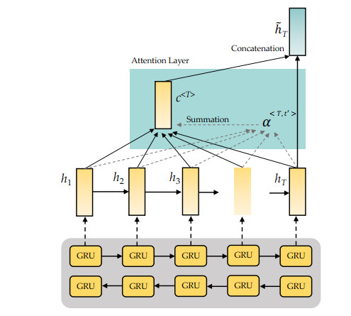
Currently, identification of complex human activities is experiencing exponential growth through the use of deep learning algorithms. Conventional strategies for recognizing human activity generally rely on handcrafted characteristics from heuristic processes in time and frequency domains. The advancement of deep learning algorithms has addressed most of these issues by automatically extracting features from multimodal sensors to correctly classify human physical activity. This study proposed an attention-based bidirectional gated recurrent unit as Att-BiGRU to enhance recurrent neural networks. This deep learning model allowed flexible forwarding and reverse sequences to extract temporal-dependent characteristics for efficient complex activity recognition. The retrieved temporal characteristics were then used to exemplify essential information through an attention mechanism. A human activity recognition (HAR) methodology combined with our proposed model was evaluated using the publicly available datasets containing physical activity data collected by accelerometers and gyroscopes incorporated in a wristwatch. Simulation experiments showed that attention mechanisms significantly enhanced performance in recognizing complex human activity.
Citation: Sakorn Mekruksavanich, Anuchit Jitpattanakul. RNN-based deep learning for physical activity recognition using smartwatch sensors: A case study of simple and complex activity recognition[J]. Mathematical Biosciences and Engineering, 2022, 19(6): 5671-5698. doi: 10.3934/mbe.2022265
Currently, identification of complex human activities is experiencing exponential growth through the use of deep learning algorithms. Conventional strategies for recognizing human activity generally rely on handcrafted characteristics from heuristic processes in time and frequency domains. The advancement of deep learning algorithms has addressed most of these issues by automatically extracting features from multimodal sensors to correctly classify human physical activity. This study proposed an attention-based bidirectional gated recurrent unit as Att-BiGRU to enhance recurrent neural networks. This deep learning model allowed flexible forwarding and reverse sequences to extract temporal-dependent characteristics for efficient complex activity recognition. The retrieved temporal characteristics were then used to exemplify essential information through an attention mechanism. A human activity recognition (HAR) methodology combined with our proposed model was evaluated using the publicly available datasets containing physical activity data collected by accelerometers and gyroscopes incorporated in a wristwatch. Simulation experiments showed that attention mechanisms significantly enhanced performance in recognizing complex human activity.

| [1] |
G. Lilis, G. Conus, N. Asadi, M. Kayal, Towards the next generation of intelligent building: An assessment study of current automation and future iot based systems with a proposal for transitional design, Sustainable Cities Soc., 28 (2017), 473–481. https://doi.org/10.1016/j.scs.2016.08.019 doi: 10.1016/j.scs.2016.08.019

|
| [2] |
B. N. Silva, M. Khan, K. Han, Towards sustainable smart cities: A review of trends, architectures, components, and open challenges in smart cities, Sustainable Cities Soc., 38 (2018), 697–713. https://doi.org/10.1016/j.scs.2018.01.053 doi: 10.1016/j.scs.2018.01.053
|
| [3] |
U. Emir, K. Ejub, M. Zakaria, A. Muhammad, B. Vanilson, Immersing citizens and things into smart cities: A social machine-based and data artifact-driven approach, Computing, 102 (2020), 1567–1586. https://doi.org/10.1007/s00607-019-00774-9 doi: 10.1007/s00607-019-00774-9
|
| [4] |
H. Zahmatkesh, F. Al-Turjman, Fog computing for sustainable smart cities in the iot era: Caching techniques and enabling technologies - an overview, Sustainable Cities Soc., 59 (2020), 102139. https://doi.org/10.1016/j.scs.2020.102139 doi: 10.1016/j.scs.2020.102139
|
| [5] |
M. M. Aborokbah, S. Al-Mutairi, A. K. Sangaiah, O. W. Samuel, Adaptive context aware decision computing paradigm for intensive health care delivery in smart cities—a case analysis, Sustainable Cities Soc., 41 (2018), 919–924. https://doi.org/10.1016/j.scs.2017.09.004 doi: 10.1016/j.scs.2017.09.004
|
| [6] | M. Al-khafajiy, L. Webster, T. Baker, A. Waraich, Towards fog driven iot healthcare: Challenges and framework of fog computing in healthcare, in Proceedings of the 2nd International Conference on Future Networks and Distributed Systems, (2018), 1–7. https://doi.org/10.1145/3231053.3231062 |
| [7] |
V. Bianchi, M. Bassoli, G. Lombardo, P. Fornacciari, M. Mordonini, I. De Munari, IoT wearable sensor and deep learning: An integrated approach for personalized human activity recognition in a smart home environment, IEEE Internet Things J., 6 (2019), 8553–8562. https://doi.org/10.1109/JIOT.2019.2920283 doi: 10.1109/JIOT.2019.2920283
|
| [8] |
P. Loprinzi, C. Franz, K. Hager, Accelerometer-assessed physical activity and depression among u.s. adults with diabetes, Ment. Health Phys. Act., 6 (2013), 79–82. https://doi.org/10.1016/j.mhpa.2013.04.003 doi: 10.1016/j.mhpa.2013.04.003
|
| [9] |
L. Coorevits, T. Coenen, The rise and fall of wearable fitness trackers, Acad. Manage., 2016 (2016), 17305. https://doi.org/10.5465/ambpp.2016.17305abstract doi: 10.5465/ambpp.2016.17305abstract
|
| [10] | F. Prinz, T. Schlange, K. Asadullah, Believe it or not: How much can we rely on published data on potential drug targets? Nat. Rev. Drug Discovery, 10 (2011), 712. https://doi.org/10.1038/nrd3439-c1 |
| [11] |
C. Jobanputra, J. Bavishi, N. Doshi, Human activity recognition: A survey, Procedia Comput. Sci., 155 (2019), 698–703. https://doi.org/10.1016/j.procs.2019.08.100 doi: 10.1016/j.procs.2019.08.100
|
| [12] |
E. Kringle, E. Knutson, L. Terhorst, Semi-supervised machine learning for rehabilitation science research, Arch. Phys. Med. Rehabil., 98 (2017), e139. https://doi.org/10.1016/j.apmr.2017.08.452 doi: 10.1016/j.apmr.2017.08.452
|
| [13] | X. Wang, D. Rosenblum, Y. Wang, Context-aware mobile music recommendation for daily activities, in Proceedings of the 20th ACM International Conference on Multimedia, (2012), 99–108. https://doi.org/10.1145/2393347.2393368 |
| [14] | N. Y. Hammerla, J. M. Fisher, P. Andras, L. Rochester, R. Walker, T. Plotz, Pd disease state assessment in naturalistic environments using deep learning, in Twenty-Ninth AAAI Conference on Artificial Intelligence, (2015), 1742–1748. Available from: https://www.aaai.org/ocs/index.php/AAAI/AAAI15/paper/view/9930. |
| [15] |
P. Ponvel, D. K. A. Singh, G. K. Beng, S. C. Chai, Factors affecting upper extremity kinematics in healthy adults: A systematic review, Crit. Rev. Phys. Rehabil. Med., 31 (2019), 101–123. https://doi.org/10.1615/CritRevPhysRehabilMed.2019030529 doi: 10.1615/CritRevPhysRehabilMed.2019030529
|
| [16] |
C. Auepanwiriyakul, S. Waibel, J. Songa, P. Bentley, A. A. Faisal, Accuracy and acceptability of wearable motion tracking for inpatient monitoring using smartwatches, Sensors, 20 (2020), 7313. https://doi.org/10.3390/s20247313 doi: 10.3390/s20247313
|
| [17] | A. R. Javed, U. Sarwar, M. Beg, M. Asim, T. Baker, H. Tawfik, A collaborative healthcare framework for shared healthcare plan with ambient intelligence, Hum.-centric Comput. Inf. Sci., 10 (2020). https://doi.org/10.1186/s13673-020-00245-7 |
| [18] |
H. Ghasemzadeh, R. Jafari, Physical movement monitoring using body sensor networks: A phonological approach to construct spatial decision trees, IEEE Trans. Ind. Inf., 7 (2011), 66–77. https://doi.org/10.1109/TII.2010.2089990 doi: 10.1109/TII.2010.2089990
|
| [19] |
A. R. Javed, L. G. Fahad, A. A. Farhan, S. Abbas, G. Srivastava, R. M. Parizin, et al., Automated cognitive health assessment in smart homes using machine learning, Sustainable Cities Soc., 65 (2021), 102572. https://doi.org/10.1016/j.scs.2020.102572 doi: 10.1016/j.scs.2020.102572
|
| [20] | S. U. Rehman, A. R. Javed, M. U. Khan, M. N. Awan, A. Farukh, A. Hussien, Personalised Comfort: A personalised thermal comfort model to predict thermal sensation votes for smart building residents, Enterp. Inf. Syst., (2020), 1–23. https://doi.org/10.1080/17517575.2020.1852316 |
| [21] |
M. Usman Sarwar, A. Rehman Javed, F. Kulsoom, S. Khan, U. Tariq, A. Kashif Bashir, Parciv: Recognizing physical activities having complex interclass variations using semantic data of smartphone, Software: Pract. Exper., 51 (2021), 532–549. https://doi.org/10.1002/spe.2846 doi: 10.1002/spe.2846
|
| [22] |
N. Alshurafa, W. Xu, J. J. Liu, M. C. Huang, B. Mortazavi, C. K. Roberts, et al., Designing a robust activity recognition framework for health and exergaming using wearable sensors, IEEE J. Biomed. Health Inf., 18 (2014), 1636–1646. https://doi.org/10.1109/JBHI.2013.2287504 doi: 10.1109/JBHI.2013.2287504
|
| [23] |
H. Arshad, M. Khan, M. Sharif, Y. Mussarat, M. Javed, Multi-level features fusion and selection for human gait recognition: An optimized framework of bayesian model and binomial distribution, Int. J. Mach. Learn. Cybern., 10 (2019), 3601–3618. https://doi.org/10.1007/s13042-019-00947-0 doi: 10.1007/s13042-019-00947-0
|
| [24] |
P. N. Dawadi, D. J. Cook, M. Schmitter-Edgecombe, Automated cognitive health assessment using smart home monitoring of complex tasks, IEEE Trans. Syst. Man Cybern. Syst., 43 (2013), 1302–1313. https://doi.org/10.1109/TSMC.2013.2252338 doi: 10.1109/TSMC.2013.2252338
|
| [25] |
S. Mekruksavanich, A. Jitpattanakul, Deep convolutional neural network with rnns for complex activity recognition using wrist-worn wearable sensor data, Electronics, 10 (2021), 1685. https://doi.org/10.3390/electronics10141685 doi: 10.3390/electronics10141685
|
| [26] |
Y. Liu, H. Yang, S. Gong, Y. Liu, X. Xiong, A daily activity feature extraction approach based on time series of sensor events, Math. Biosci. Eng., 17 (2020), 5173–5189. https://doi.org/10.3934/mbe.2020280 doi: 10.3934/mbe.2020280
|
| [27] | D. Anguita, A. Ghio, L. Oneto, X. Parra, J. L. Reyes-Ortiz, Human activity recognition on smartphones using a multiclass hardware-friendly support vector machine, in Ambient Assisted Living and Home Care, (2012), 216–223. https://doi.org/10.1007/978-3-642-35395-6_30 |
| [28] |
O. Lara, M. Labrador, A survey on human activity recognition using wearable sensors, IEEE Commun. Surv. Tutorials, 15 (2013), 1192–1209. https://doi.org/10.1109/SURV.2012.110112.00192 doi: 10.1109/SURV.2012.110112.00192
|
| [29] |
S. Liu, J. Wang, W. Zhang, Federated personalized random forest for human activity recognition, Math. Biosci. Eng., 19 (2022), 953–971. https://doi.org/10.3934/mbe.2022044 doi: 10.3934/mbe.2022044
|
| [30] |
O. Russakovsky, J. Deng, H. Su, J. Krause, S. Satheesh, S. Ma, et al., Imagenet large scale visual recognition challenge, Int. J. Comput. Vision, 115 (2015), 211–252. https://doi.org/10.1007/s11263-015-0816-y doi: 10.1007/s11263-015-0816-y
|
| [31] | J. Devlin, M. Chang, K. Lee, K. Toutanova, BERT: Pre-training of deep bidirectional transformers for language understanding, preprint, arXiv: 1810.04805. |
| [32] | Y. Lecun, Y. Bengio, G. Hinton, Deep learning, Nature, 521 (2015), 436–444. https://doi.org/10.1038/nature14539 |
| [33] |
A. Murad, J. Y. Pyun, Deep recurrent neural networks for human activity recognition, Sensors, 17 (2017), 2556. https://doi.org/10.3390/s17112556 doi: 10.3390/s17112556
|
| [34] |
O. Nafea, W. Abdul, G. Muhammad, M. Alsulaiman, Sensor-based human activity recognition with spatio-temporal deep learning, Sensors, 21 (2021), 2141. https://doi.org/10.3390/s21062141 doi: 10.3390/s21062141
|
| [35] |
V. Y. Senyurek, M. H. Imtiaz, P. Belsare, S. Tiffany, E. Sazonov, A cnn-lstm neural network for recognition of puffing in smoking episodes using wearable sensors, Biomed. Eng. Lett., 10 (2020), 195–203. https://doi.org/10.1007/s13534-020-00147-8 doi: 10.1007/s13534-020-00147-8
|
| [36] |
X. Liu, M. Chen, T. Liang, C. Lou, H. Wang, X. Liu, A lightweight double-channel depthwise separable convolutional neural network for multimodal fusion gait recognition, Math. Biosci. Eng., 19 (2022), 1195–1212. https://doi.org/10.3934/mbe.2022055 doi: 10.3934/mbe.2022055
|
| [37] | S. Dernbach, B. Das, N. C. Krishnan, B. L. Thomas, D. J. Cook, Simple and complex activity recognition through smart phones, in 2012 8th International Conference on Intelligent Environments, (2012), 214–221. https://doi.org/10.1109/IE.2012.39 |
| [38] | T. Huynh, M. Fritz, B. Schiele, Discovery of activity patterns using topic models, in 10th International Conference on Ubiquitous Computing, (2008), 10–19. https://doi.org/10.1145/1409635.1409638 |
| [39] |
L. Liu, Y. Peng, S. Wang, M. Liu, Z. Huang, Complex activity recognition using time series pattern dictionary learned from ubiquitous sensors, Inf. Sci., 340-341 (2016), 41–57. https://doi.org/10.1016/j.ins.2016.01.020 doi: 10.1016/j.ins.2016.01.020
|
| [40] |
L. Peng, L. Chen, M. Wu, G. Chen, Complex activity recognition using acceleration, vital sign, and location data, IEEE Trans. Mobile Comput., 18 (2019), 1488–1498. https://doi.org/10.1109/TMC.2018.2863292 doi: 10.1109/TMC.2018.2863292
|
| [41] |
T. Y. Kim, S. B. Cho, Predicting residential energy consumption using cnn-lstm neural networks, Energy, 182 (2019), 72–81. https://doi.org/10.1016/j.energy.2019.05.230 doi: 10.1016/j.energy.2019.05.230
|
| [42] | S. Hochreiter, J. Schmidhuber, Long short-term memory, Neural Comput., 9 (1997), 1735–1780. https://doi.org/10.1162/neco.1997.9.8.1735 |
| [43] | Y. Chen, K. Zhong, J. Zhang, Q. Sun, X. Zhao, Lstm networks for mobile human activity recognition, in Proceedings of the 2016 International Conference on Artificial Intelligence: Technologies and Applications, (2016), 50–53. https://doi.org/10.2991/icaita-16.2016.13 |
| [44] |
F. Moya Rueda, R. Grzeszick, G. A. Fink, S. Feldhorst, M. Ten Hompel, Convolutional neural networks for human activity recognition using body-worn sensors, Informatics, 5 (2018), 26. https://doi.org/10.3390/informatics5020026 doi: 10.3390/informatics5020026
|
| [45] | J. Bi, X. Zhang, H. Yuan, J. Zhang, M. Zhou, A hybrid prediction method for realistic network traffic with temporal convolutional network and lstm, IEEE Trans. Autom. Sci. Eng., (2021), 1–11. https://doi.org/10.1109/TASE.2021.3077537 |
| [46] |
F. J. Ordóñez, D. Roggen, Deep convolutional and lstm recurrent neural networks for multimodal wearable activity recognition, Sensors, 16 (2016), 115. https://doi.org/10.3390/s16010115 doi: 10.3390/s16010115
|
| [47] |
K. Xia, J. Huang, H. Wang, Lstm-cnn architecture for human activity recognition, IEEE Access, 8 (2020), 56855–56866. https://doi.org/10.1109/ACCESS.2020.2982225 doi: 10.1109/ACCESS.2020.2982225
|
| [48] |
M. Ronald, A. Poulose, D. S. Han, iSPLInception: An inception-resnet deep learning architecture for human activity recognition, IEEE Access, 9 (2021), 68985–69001. https://doi.org/10.1109/ACCESS.2021.3078184 doi: 10.1109/ACCESS.2021.3078184
|
| [49] |
R. Huan, Z. Zhan, L. Ge, K. Chi, P. Chen, R. Liang, A hybrid cnn and blstm network for human complex activity recognition with multi-feature fusion, Multimedia Tools Appl., 80 (2021), 36159–36182. https://doi.org/10.1007/s11042-021-11363-4 doi: 10.1007/s11042-021-11363-4
|
| [50] | X. Zhang, M. Lapata, Chinese poetry generation with recurrent neural networks, in Proceedings of the 2014 Conference on Empirical Methods in Natural Language Processing (EMNLP), (2014), 670–680. https://doi.org/10.3115/v1/D14-1074 |
| [51] | Q. Wang, T. Luo, D. Wang, C. Xing, Chinese song iambics generation with neural attention-based model, preprint, arXiv: 1604.06274. |
| [52] | Q. Chen, X. Zhu, Z. H. Ling, S. Wei, H. Jiang, D. Inkpen, Enhanced lstm for natural language inference, in Proceedings of the 55th Annual Meeting of the Association for Computational Linguistics, 1 (2017), 1657–1668. https://doi.org/10.18653/v1/P17-1152 |
| [53] | V. K. Tran, L. M. Nguyen, Semantic refinement gru-based neural language generation for spoken dialogue systems, in Computational Linguistics, (2018), 63–75. https://doi.org/10.1007/978-981-10-8438-6_6 |
| [54] | T. Bansal, D. Belanger, A. McCallum, Ask the gru: Multi-task learning for deep text recommendations, in Proceedings of the 10th ACM Conference on Recommender Systems, (2016), 107–114. https://doi.org/10.1145/2959100.2959180 |
| [55] | A. Graves, N. Jaitly, A. R. Mohamed, Hybrid speech recognition with deep bidirectional lstm, in 2013 IEEE Workshop on Automatic Speech Recognition and Understanding, (2013), 273–278. https://doi.org/10.1109/ASRU.2013.6707742 |
| [56] | K. Cho, B. van Merrienboer, C. Gulcehre, F. Bougares, H. Schwenk, Y. Bengio, Learning phrase representations using rnn encoder-decoder for statistical machine translation, preprient, arXiv: 1406.1078. |
| [57] | D. Singh, E. Merdivan, I. Psychoula, J. Kropf, S. Hanke, M. Geist, et al., Human activity recognition using recurrent neural networks, in Machine Learning and Knowledge Extraction, (2017), 267–274. https://doi.org/10.1007/978-3-319-66808-6_18 |
| [58] |
M. Schuster, K. Paliwal, Bidirectional recurrent neural networks, IEEE Trans. Signal Process., 45 (1997), 2673–2681. https://doi.org/10.1109/78.650093 doi: 10.1109/78.650093
|
| [59] | L. Alawneh, B. Mohsen, M. Al-Zinati, A. Shatnawi, M. Al-Ayyoub, A comparison of unidirectional and bidirectional lstm networks for human activity recognition, in 2020 IEEE International Conference on Pervasive Computing and Communications Workshops (PerCom Workshops), (2020), 1–6. https://doi.org/10.1109/PerComWorkshops48775.2020.9156264 |
| [60] |
S. Mekruksavanich, A. Jitpattanakul, Lstm networks using smartphone data for sensor-based human activity recognition in smart homes, Sensors, 21 (2021), 1636. https://doi.org/10.3390/s21051636 doi: 10.3390/s21051636
|
| [61] |
J. Wu, J. Wang, A. Zhan, C. Wu, Fall detection with cnn-casual lstm network, Information, 12 (2021), 403. https://doi.org/10.3390/info12100403 doi: 10.3390/info12100403
|
| [62] | K. Cho, B. van Merriënboer, D. Bahdanau, Y. Bengio, On the properties of neural machine translation: Encoder-decoder approaches, preprient, arXiv: 1409.1259. |
| [63] | J. Chung, C. Gulcehre, K. Cho, Y. Bengio, Empirical evaluation of gated recurrent neural networks on sequence modeling, preprient, arXiv: 1412.3555. |
| [64] |
M. Quadrana, P. Cremonesi, D. Jannach, Sequence-aware recommender systems, ACM Comput. Surv., 51 (2019), 1–36. https://doi.org/10.1145/3190616 doi: 10.1145/3190616
|
| [65] | S. Rendle, C. Freudenthaler, L. Schmidt-Thieme, Factorizing personalized markov chains for next-basket recommendation, in Proceedings of the 19th International Conference on World Wide Web, (2010), 811–820. https://doi.org/10.1145/1772690.1772773 |
| [66] | J. Okai, S. Paraschiakos, M. Beekman, A. Knobbe, C. R. de Sá, Building robust models for human activity recognition from raw accelerometers data using gated recurrent units and long short term memory neural networks, in 2019 41st Annual International Conference of the IEEE Engineering in Medicine and Biology Society (EMBC), (2019), 2486–2491. https://doi.org/10.1109/EMBC.2019.8857288 |
| [67] |
H. M. Lynn, S. B. Pan, P. Kim, A deep bidirectional gru network model for biometric electrocardiogram classification based on recurrent neural networks, IEEE Access, 7 (2019), 145395–145405. https://doi.org/10.1109/ACCESS.2019.2939947 doi: 10.1109/ACCESS.2019.2939947
|
| [68] | T. Alsarhan, L. Alawneh, M. Al-Zinati, M. Al-Ayyoub, Bidirectional gated recurrent units for human activity recognition using accelerometer data, in 2019 IEEE SENSORS, (2019), 1–4. https://doi.org/10.1109/SENSORS43011.2019.8956560 |
| [69] |
L. Alawneh, T. Alsarhan, M. Al-Zinati, M. Al-Ayyoub, Y. Jararweh, H. Lu, Enhancing human activity recognition using deep learning and time series augmented data, J. Ambient Intell. Humanized Comput., 12 (2021), 10565–10580. https://doi.org/10.1007/s12652-020-02865-4 doi: 10.1007/s12652-020-02865-4
|
| [70] |
C. Xu, D. Chai, J. He, X. Zhang, S. Duan, Innohar: A deep neural network for complex human activity recognition, IEEE Access, 7 (2019), 9893–9902. https://doi.org/10.1109/ACCESS.2018.2890675 doi: 10.1109/ACCESS.2018.2890675
|
| [71] | V. S. Murahari, T. Plötz, On attention models for human activity recognition, in Proceedings of the 2018 ACM International Symposium on Wearable Computers, 2018,100–103. https://doi.org/10.1145/3267242.3267287 |
| [72] | P. Li, Y. Song, I. V. McLoughlin, W. Guo, L. R. Dai, An attention pooling based representation learning method for speech emotion recognition, in Proc. Interspeech 2018, (2018), 3087–3091. https://doi.org/10.21437/Interspeech.2018-1242 |
| [73] | C. Raffel, D. P. W. Ellis, Feed-forward networks with attention can solve some long-term memory problems, preprient, arXiv: 1512.08756. |
| [74] | M. N. Haque, M. T. H. Tonmoy, S. Mahmud, A. A. Ali, M. Asif Hossain Khan, M. Shoyaib, Gru-based attention mechanism for human activity recognition, in 2019 1st International Conference on Advances in Science, Engineering and Robotics Technology (ICASERT), (2019), 1–6. https://doi.org/10.1109/ICASERT.2019.8934659 |
| [75] |
L. Peng, L. Chen, Z. Ye, Y. Zhang, Aroma: A deep multi-task learning based simple and complex human activity recognition method using wearable sensors, Proc. ACM Interact., Mobile, Wearable Ubiquitous Technol., 2 (2018), 1–16. https://doi.org/10.1145/3214277 doi: 10.1145/3214277
|
| [76] |
E. Kim, S. Helal, D. Cook, Human activity recognition and pattern discovery, IEEE Pervasive Comput., 9 (2010), 48–53. https://doi.org/10.1109/MPRV.2010.7 doi: 10.1109/MPRV.2010.7
|
| [77] |
L. Liu, Y. Peng, M. Liu, Z. Huang, Sensor-based human activity recognition system with a multilayered model using time series shapelets, Knowledge-Based Syst., 90 (2015), 138–152. https://doi.org/10.1016/j.knosys.2015.09.024 doi: 10.1016/j.knosys.2015.09.024
|
| [78] | D. Anguita, A. Ghio, L. Oneto, X. Parra, J. L. Reyes-Ortiz, A public domain dataset for human activity recognition using smartphones, in Proceedings of the 21th International European Symposium on Artificial Neural Networks, Computational Intelligence and Machine Learning, (2013), 437–442. Available from: http://hdl.handle.net/2117/20897. |
| [79] |
Y. F. Zhang, P. J. Thorburn, W. Xiang, P. Fitch, SSIM—A deep learning approach for recovering missing time series sensor data, IEEE Internet Things J., 6 (2019), 6618–6628. https://doi.org/10.1109/JIOT.2019.2909038 doi: 10.1109/JIOT.2019.2909038
|
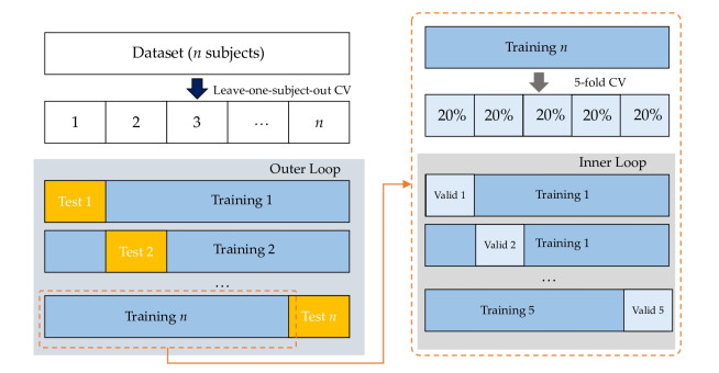
| [80] | G. C. Cawley, N. L. Talbot, On over-fitting in model selection and subsequent selection bias in performance evaluation, J. Mach. Learn. Res., 11 (2010), 2079–2107. Available from: https://www.jmlr.org/papers/volume11/cawley10a/cawley10a. |
| [81] |
S. Parvandeh, H. W. Yeh, M. P. Paulus, B. A. McKinney, Consensus features nested cross-validation, Bioinformatics, 36 (2020), 3093–3098. https://doi.org/10.1093/bioinformatics/btaa046 doi: 10.1093/bioinformatics/btaa046
|
| [82] |
S. Varma, R. Simon, Bias in error estimation when using cross-validation for model selection, BMC Bioinf., 7 (2006), 91. https://doi.org/10.1186/1471-2105-7-91 doi: 10.1186/1471-2105-7-91
|
| [83] | D. Anguita, A. Ghio, L. Oneto, X. Parra, J. L. Reyes-Ortiz, Energy efficient smartphone-based activity recognition using fixed-point arithmetic, J. Univers. Comput. Sci., 19 (2013), 1295–1314. Available from: http://hdl.handle.net/2117/20437. |
| [84] | A. Reiss, D. Stricker, Introducing a new benchmarked dataset for activity monitoring, in 2012 16th International Symposium on Wearable Computers, (2012), 108–109. https://doi.org/10.1109/ISWC.2012.13 |
| [85] | D. Roggen, A. Calatroni, M. Rossi, T. Holleczek, K. Förster, G. Tröster, et al., Collecting complex activity datasets in highly rich networked sensor environments, in 2010 Seventh International Conference on Networked Sensing Systems (INSS), (2010), 233–240. https://doi.org/10.1109/INSS.2010.5573462 |
| [86] | T. Luong, H. Pham, C. D. Manning, Effective approaches to attention-based neural machine translation, in Proceedings of the 2015 Conference on Empirical Methods in Natural Language Processing, (2015), 1412–1421. https://doi.org/10.18653/v1/D15-1166 |
| [87] |
I. C. Gyllensten, A. G. Bonomi, Identifying types of physical activity with a single accelerometer: Evaluating laboratory-trained algorithms in daily life, IEEE Trans. Biomed. Eng., 58 (2011), 2656–2663. https://doi.org/10.1109/TBME.2011.2160723 doi: 10.1109/TBME.2011.2160723
|
Figures(9) / Tables(7)

Sakorn Mekruksavanich, Anuchit Jitpattanakul. RNN-based deep learning for physical activity recognition using smartwatch sensors: A case study of simple and complex activity recognition[J]. Mathematical Biosciences and Engineering, 2022, 19(6): 5671-5698. doi: 10.3934/mbe.2022265


 DownLoad: