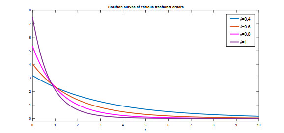
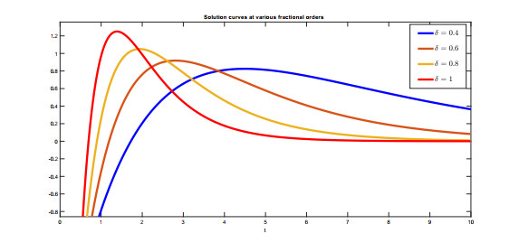
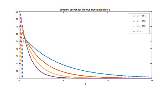
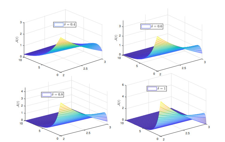
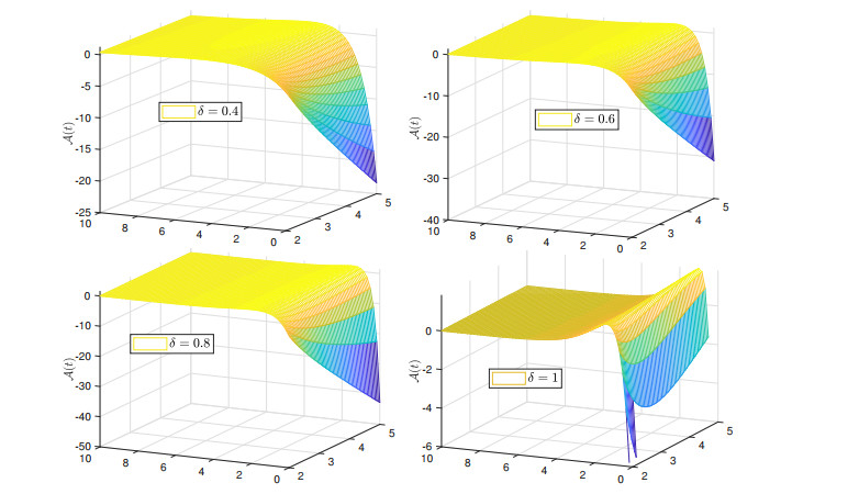
Recently, non-singular fractional operators have a significant role in the modeling of real-world problems. Specifically, the Caputo-Fabrizio operators are used to study better dynamics of memory processes. In this paper, under the non-singular fractional operator with exponential decay kernel, we analyze the Ambartsumian equation qualitatively and computationally. We deduce the result of the existence of at least one solution to the proposed equation through Krasnoselskii's fixed point theorem. Also, we utilize the Banach fixed point theorem to derive the result concerned with unique solution. We use the concept of functional analysis to show that the proposed equation is Ulam-Hyers and Ulam-Hyers-Rassias stable. We use an efficient analytical approach to compute a semi-analytical solution to the proposed problem. The convergence of the series solution to an exact solution is proved through non-linear analysis. Lastly, we present the solution for different fractional orders.
Citation: Shabir Ahmad, Aman Ullah, Ali Akgül, Manuel De la Sen. A study of fractional order Ambartsumian equation involving exponential decay kernel[J]. AIMS Mathematics, 2021, 6(9): 9981-9997. doi: 10.3934/math.2021580
Recently, non-singular fractional operators have a significant role in the modeling of real-world problems. Specifically, the Caputo-Fabrizio operators are used to study better dynamics of memory processes. In this paper, under the non-singular fractional operator with exponential decay kernel, we analyze the Ambartsumian equation qualitatively and computationally. We deduce the result of the existence of at least one solution to the proposed equation through Krasnoselskii's fixed point theorem. Also, we utilize the Banach fixed point theorem to derive the result concerned with unique solution. We use the concept of functional analysis to show that the proposed equation is Ulam-Hyers and Ulam-Hyers-Rassias stable. We use an efficient analytical approach to compute a semi-analytical solution to the proposed problem. The convergence of the series solution to an exact solution is proved through non-linear analysis. Lastly, we present the solution for different fractional orders.

| [1] | V. A. Ambartsumian, On the fluctuation of the brightness of the milky way, Dokl. Akad. Nauk. USSR, 44 (1994), 223-226. |
| [2] | T. Kato, J. B. McLeod, The functional-differential equation y0(x) = ay(lx) + by(x), B. Am. Math. Soc., 77 (1971), 891-935. |
| [3] | J. Patade, S. Bhalekar, On analytical solution of Ambartsumian equation, Natl. Acad. Sci. Lett., 40 (2017), 291–293. |
| [4] | V. Daftardar-Gejji, S. Bhalekar, Solving fractional diffusion-wave equations using the new iterative method, Fract. Calc. Appl. Anal., 11 (2008), 193-202. |
| [5] | H. Fatoorehchi, H. Abolghasemi, Finding all real roots of a polynomial by matrix algebra and the Adomian decomposition method, J. Egypt. Math. Soc., 22 (2014), 524-528. |
| [6] | A. Alshaery, A. Ebaid, Accurate analytical periodic solution of the elliptical Kepler equation using the Adomian decomposition method, Acta Astronaut., 140 (2017), 27-33. |
| [7] | Y. Cherruault, G. Adomian, Decompostion methods: a new proof of convergence, Math. Comput. Model., 18 (1993), 103-106. |
| [8] | H. O. Bakodah, A. Ebaid, Exact solution of Ambartsumian delay differential equation and comparison with Daftardar-Gejji and Jafari approximate method, Mathematics, 6 (2018), 331. |
| [9] | A. A. Alatawi, M. Aljoufi, F. M. Alharbi, A. Ebaid, Investigation of the surface brightness model in the milky way via homotopy perturbation method, J. Appl. Math. Phys., 8 (2020), 434-442. |
| [10] | D. Kumar, J. Singh, D. Baleanu, S. Rathore. Analysis of a fractional model of the Ambartsumian equation, Eur. Phys. J. Plus, 133 (2018), 259. |
| [11] | A. A. Kilbas, H. Srivastava, J. J. Trujillo, Theory and application of fractional differential equations, North Holland Mathematics Studies, Amsterdam: Elseveir, 204 (2006), 1–523. |
| [12] | M. M. Khader, K. M. Saad, Z. Hammouch, D. Baleanu, A spectral collocation method for solving fractional KdV and KdV-Burgers equations with non-singular kernel derivatives, Appl. Numer. Math., 161 (2021), 137–146. |
| [13] |
K. M. Saad, M. Alqhtani, Numerical simulation of the fractal-fractional reaction diffusion equations with general nonlinear, AIMS Mathematics, 6 (2021), 3788–3804. doi: 10.3934/math.2021225

|
| [14] | K. M. Saad, E. H. F. AL-Sharif, Comparative study of a cubic autocatalytic reaction via different analysis methods, Discrete Cont. Dyn. S, 12 (2019), 665–684. |
| [15] | A. Shah, R. A. Khan, A. Khan, H. Khan, J. F. Gómez-Aguilar, Investigation of a system of nonlinear fractional order hybrid differential equations under usual boundary conditions for existence of solution, Math. Methods Appl. Sci., 44 (2021), 1628–1638. |
| [16] | H. Khan, J. F. Gomez-Aguilar, T. Abdeljawad, A. Khan, Existence results and stability criteria for ABC-fuzzy-Volterra integro-differential equation, Fractals, 28 (2020), 2040048. |
| [17] | A. Khan, H. Khan, J. F. Gómez-Aguilar, T. Abdeljawad, Existence and Hyers-Ulam stability for a nonlinear singular fractional differential equations with Mittag-Leffler kernel, Chaos Soliton. Fract., 127 (2019), 422–427. |
| [18] | T. Abdeljawad, A. Atangana, J. F. Gómez-Aguilar, F. Jarad, On a more general fractional integration by parts formulae and applications, Physica A., 536 (2019), 122494. |
| [19] | A. Ullah, T. Abdeljawad, S. Ahmad, K. Shah, Study of a fractional-order epidemic model of childhood diseases, J. Funct. Space., 2020 (2020), 5895310. |
| [20] | K. K. Nisar, S. Ahmad, A. Ullah, K. Shah, H. Alrabaiah, M. Arfan, Mathematical analysis of SIRD model of COVID-19 with Caputo fractional derivative based on real data, Results Phys., 21 (2021) 103772. |
| [21] | R. A. Khan, K. Shah, Existence and uniqueness of solutions to fractional order multi-point boundary value problems, Commun. Appl. Anal., 19 (2015), 515-526. |
| [22] |
K. Shah, M. A. Alqudah, F. Jarad, T. Abdeljawad, Semi-analytical study of Pine Wilt Disease model with convex rate under Caputo-Fabrizio fractional order derivative, Chaos Soliton. Fract., 135 (2020), 109754. doi: 10.1016/j.chaos.2020.109754
|
| [23] | M. Caputo, M. Fabrizio, A new definition of fractional derivative without singular kernel, Progr. Fract. Differ. Appl., 1 (2015), 73–85. |
| [24] | V. F. Morales-Delgado, M. A. Taneco-Hernández, J. F. Gómez-Aguilar, On the solutions of fractional order of evolution equations, Eur. Phys. J. Plus., 132 (2017), 47. |
| [25] | L. X. Vivas-Cruz, A. González-Calderón, M. A. Taneco-Hernández, D. P. Luis, Theoretical analysis of a model of fluid flow in a reservoir with the Caputo-Fabrizio operator, Commun. Nonlinear Sci., 84 (2020), 105186. |
| [26] | D. Baleanu, A. Jajarmi, H. Mohammadi, S. Rezapour, A new study on the mathematical modelling of human liver with Caputo-Fabrizio fractional derivative, Chaos Soliton. Fract., 134 (2020), 109705. |
| [27] | D. Baleanu, H. Mohammadi, S. Rezapour, A mathematical theoretical study of a particular system of Caputo-Fabrizio fractional differential equations for the Rubella disease model, Adv. Differ. Equ., 2020 (2020), 184. |
| [28] |
F. Gao, X. L. Li, W. Q. Li, X. J. Zhou, Stability analysis of a fractional-order novel hepatitis B virus model with immune delay based on Caputo-Fabrizio derivative, Chaos Soliton. Fract., 142 (2021), 110436. doi: 10.1016/j.chaos.2020.110436
|
| [29] | S. Ahmad, A. Ullah, K. Shah, A. Akgül, Computational analysis of the third order dispersive fractional PDE under exponential-decay and Mittag-Leffler type kernels, Numer. Meth. Part. D. E., 2020, DOI: 10.1002/num.22627. |
| [30] | R. K. Pandey, H. K. Mishra, Homotopy analysis Sumudu transform method for time\textemdash Fractional third order dispersive partial differential equation, Adv. Comput. Math., 43 (2017), 365-383. |
| [31] |
D. Baleanu, B. Shiri, Collocation methods for fractional differential equations involving non-singular kernel, Chaos Soliton. Fract., 116 (2018), 136-145. doi: 10.1016/j.chaos.2018.09.020
|
| [32] | H. Jafari, C. M. Khalique, M. Nazari, Application of the Laplace decomposition method for solving linear and nonlinear fractional diffusion-wave equations, Appl. Math. Lett., 24 (2011), 1799-1805. |
| [33] | M. Z. Mohamed, T. M. Elzaki, Comparison between the Laplace decomposition method and Adomian decomposition in time-space fractional nonlinear fractional differential equations, Appl. Math., 9 (2018), 448–458. |
| [34] |
K. Shah, F. Jarad, T. Abdeljawad, On a nonlinear fractional order model of dengue fever disease under Caputo-Fabrizio derivative, Alex. Eng. J., 59 (2020), 2305–2313. doi: 10.1016/j.aej.2020.02.022
|
| [35] | M. Sher, K. Shah, Z. A. Khan, H. Khan, A. Khan, Computational and theoretical modeling of the transmission dynamics of novel COVID-19 under Mittag-Leffler Power Law, Alexandria Eng. J. 59 (2020), 3133–3147. |
| [36] | D. H. Hyers, On the stability of the linear functional equation, Proc. Natl. Acad. Sci. USA, 27 (1941), 222-224. |
| [37] |
T. M. Rassias, On the stability of the linear mapping in Banach spaces, P. Am. Math. Soc., 72 (1978), 297-300. doi: 10.1090/S0002-9939-1978-0507327-1
|
| [38] |
A. Khan, H. Khan, J. F. Gomez-Aguilar, T. Abdeljawad, Existence and Hyers-Ulam stability for a nonlinear singular fractional differential equations with Mittag-Leffler kernel, Chaos Soliton. Fract., 127 (2019), 422-427. doi: 10.1016/j.chaos.2019.07.026
|
| [39] |
H. Khan, T. Abdeljawad, M. Aslam, R. A. Khan, A. Khan, Existence of positive solution and HyersUlam stability for a nonlinear singular-delay-fractional differential equation, Adv. Differ. Equ., 2019 (2019), 104. doi: 10.1186/s13662-019-2054-z
|
| [40] | T. A. Burton, T. Furumochi, Krasnoselskiis fixed point theorem and stability, Nonlinear Anal.-Theor., 49 (2002), 445–454. |

Figures(6)

Shabir Ahmad, Aman Ullah, Ali Akgül, Manuel De la Sen. A study of fractional order Ambartsumian equation involving exponential decay kernel[J]. AIMS Mathematics, 2021, 6(9): 9981-9997. doi: 10.3934/math.2021580


 DownLoad: