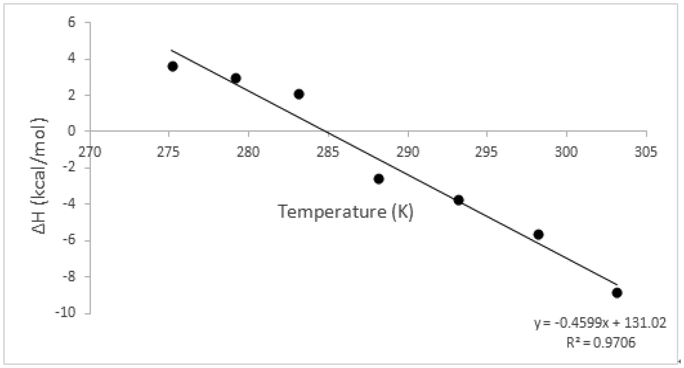
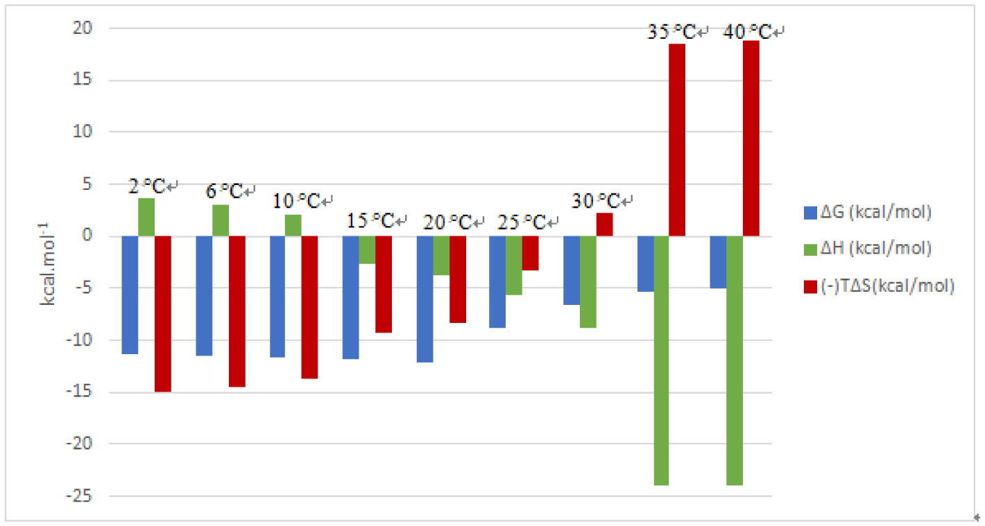
An entropically-driven binding interaction at a certain temperature may change to an enthalpically-driven process at another temperature, depending on the polarization state of the groups that are involved in binding. The streptavidin-biotin complex has been extensively studied across biological, medical, chemical and material science fields using various techniques, however, not much has been reported on this interaction across a broad temperature range, between 2 °C and 40 °C using biophysical techniques. In this study, we determined how the forces involved in the streptavidin-biotin complex formation are affected by the reaction temperature using the Affinity ITC (TA Instruments). We observed that this complex formation is a spontaneous binding process, indicated by a negative Gibbs energy (ΔG) at all temperatures tested. The observed negative heat capacity (ΔCp) ∼ −459.9 cal/mol K highlights the polar solvation of the interaction that corresponds to a decreasing enthalpy (more negative) (ΔH) with increasing reaction temperature. The stoichiometry (n) of 0.98 was estimated at 25 °C. An increase in reaction temperature resulted in an almost two-fold increase or more in n, notably from 1.59 to 3.41 between 30 °C and 40 °C. Whereas, at lower reaction temperatures, 2 °C to 10 °C, higher molar binding ratios were recorded, i.e. 2.74 to 5.76. We report an enthalpically-driven interaction between 30 °C and 40 °C whereas, an entropically-favourable interaction is observed at lower temperatures, suggestive of an interaction dominated by nonpolar interactions at lower temperatures and polar interactions at higher temperatures. Consequently, alterations in the polarisation state of streptavidin result in moderate binding affinity of biotin to streptavidin at higher reaction temperatures, KD 10−4 ≤ 10−5 M.
Citation: Keleabetswe L. Mpye, Samantha Gildenhuys, Salerwe Mosebi. The effects of temperature on streptavidin-biotin binding using affinity isothermal titration calorimetry[J]. AIMS Biophysics, 2020, 7(4): 236-247. doi: 10.3934/biophy.2020018
An entropically-driven binding interaction at a certain temperature may change to an enthalpically-driven process at another temperature, depending on the polarization state of the groups that are involved in binding. The streptavidin-biotin complex has been extensively studied across biological, medical, chemical and material science fields using various techniques, however, not much has been reported on this interaction across a broad temperature range, between 2 °C and 40 °C using biophysical techniques. In this study, we determined how the forces involved in the streptavidin-biotin complex formation are affected by the reaction temperature using the Affinity ITC (TA Instruments). We observed that this complex formation is a spontaneous binding process, indicated by a negative Gibbs energy (ΔG) at all temperatures tested. The observed negative heat capacity (ΔCp) ∼ −459.9 cal/mol K highlights the polar solvation of the interaction that corresponds to a decreasing enthalpy (more negative) (ΔH) with increasing reaction temperature. The stoichiometry (n) of 0.98 was estimated at 25 °C. An increase in reaction temperature resulted in an almost two-fold increase or more in n, notably from 1.59 to 3.41 between 30 °C and 40 °C. Whereas, at lower reaction temperatures, 2 °C to 10 °C, higher molar binding ratios were recorded, i.e. 2.74 to 5.76. We report an enthalpically-driven interaction between 30 °C and 40 °C whereas, an entropically-favourable interaction is observed at lower temperatures, suggestive of an interaction dominated by nonpolar interactions at lower temperatures and polar interactions at higher temperatures. Consequently, alterations in the polarisation state of streptavidin result in moderate binding affinity of biotin to streptavidin at higher reaction temperatures, KD 10−4 ≤ 10−5 M.

| [1] | González M, Bagatolli LA, Echabe I, et al. (1997) Interaction of biotin with streptavidin. Thermostability and conformational changes upon binding. J Biol Chem 272: 11288-11294. |
| [2] | Wilchek M, Bayer EA (1990) Introduction to avidin-biotin technology. Methods Enzymol 184: 5-13. |
| [3] | Kurzban GP, Gitlin G, Bayer EA, et al. (1990) Biotin binding changes the conformation and decreases tryptophan accessibility of streptavidin. J Protein Chem 9: 673-682. |
| [4] | Green NM (1990) Streptomyces avidinii. Methods Enzymol 184: 51-67. |
| [5] | Delgadillo RF, Mueser TC, Zaleta-Rivera K, et al. (2019) Detailed characterization of the solution kinetics and thermodynamics of biotin, biocytin and HABA binding to avidin and streptavidin. Plos One 14: e0204194. |
| [6] | Hyre DE, Stayton PS, Trong IL, et al. (2000) Ser45 plays an important role in managing both the equilibrium and transition state energetics of the streptavidin-biotin system. Protein Sci 9: 878-885. |
| [7] | Chilkoti A, Tan PH, Stayton PS (1995) Site-directed mutagenesis studies of the high-affinity streptavidin-biotin complex: Contributions of tryptophan residues 79, 108, and 120. Proc Natl Acad Sci 92: 1754-1758. |
| [8] | Klumb LA, Chu V, Stayton PS (1998) Energetic roles of hydrogen bonds at the ureido oxygen binding pocket in the streptavidin-biotin complex. Biochemistry 37: 7657-7663. |
| [9] | Qureshi MH, Yeung JC, Wu SC, et al. (2001) Development and characterization of a series of soluble tetrameric and monomeric streptavidin muteins with differential biotin binding affinities. J Biol Chem 276: 46422-46428. |
| [10] | Laitinen OH, Nordlund HR, Hytönen VP, et al. (2003) Rational design of an active avidin monomer. J Biol Chem 278: 4010-4014. |
| [11] | Diamandis EP, Christopoulos TK (1991) The biotin-(strept) avidin system: principles and applications in biotechnology. Clin Chem 37: 625-636. |
| [12] | Sano T, Glazer AN, Cantor CR (1992) A streptavidin-metallothionein chimera that allows specific labeling of biological materials with many different heavy metal ions. Proc Natl Acad Sci 89: 1534-1538. |
| [13] | Chaiet L, Miller TW, Tausig F, et al. (1963) Antibiotic MSD-235. II. separation and purification of synergistic components. Antimicrob Agents Chemother 161: 28-32. |
| [14] | Green NM (1975) Avidin. Adv Protein Chem 29: 85-133. |
| [15] | Kuo TC, Tsai CW, Lee PC, et al. (2015) Revisiting the streptavidin-biotin binding by using an aptamer and displacement isothermal calorimetry titration. J Mol Recognit 28: 125-128. |
| [16] | Pérez-Luna VH, O'Brien MJ, Opperman KA, et al. (1999) Molecular recognition between genetically engineered streptavidin and surface-bound biotin. J Am Chem Soc 121: 6469-6478. |
| [17] | Lo YS, Simons J, Beebe TP (2002) Temperature dependence of the biotin−avidin bond-rupture force studied by atomic force microscopy. J Phys Chem B 106: 9847-9852. |
| [18] | Neish CS, Martin IL, Henderson RM, et al. (2002) Direct visualization of ligand-protein interactions using atomic force microscopy. Br J Pharmacol 135: 1943-1950. |
| [19] | Liu F, Zhang JZH, Mei Y (2016) The origin of the cooperativity in the streptavidin-biotin system: A computational investigation through molecular dynamics simulations. Sci Rep 6: 27190. |
| [20] | Green N (1966) Thermodynamics of the binding of biotin and some analogues by avidin. Biochem J 101: 774-780. |
| [21] | Du X, Li Y, Xia YL, et al. (2016) Insights into protein–ligand interactions: Mechanisms, models, and methods. Int J Mol Sci 17: 1-34. |
| [22] | Bouchemal K (2008) New challenges for pharmaceutical formulations and drug delivery systems characterization using isothermal titration calorimetry. Drug Discov Today 13: 960-972. |
| [23] | Roselin LS, Lin M-S, Lin PH, et al. (2010) Recent trends and some applications of isothermal titration calorimetry in biotechnology. Biotechnol J 5: 85-98. |
| [24] | Velazquez-Campoy A, Ohtaka H, Nezami A, et al. (2004) Isothermal titration calorimetry. Curr Protoc Cell Biol 23: 17.81-17.8.24. |
| [25] | Velazquez-Campoy A, Freire E (2006) Isothermal titration calorimetry to determine association constants for high-affinity ligands. Nat Protoc 1: 186-191. |
| [26] | Kuo TC, Lee PC, Tsai CW, et al. (2013) Salt bridge exchange binding mechanism between streptavidin and its DNA aptamer--thermodynamics and spectroscopic evidences. J Mol Recognit 26: 149-159. |
| [27] | Rajarathnam K, Rosgen J (2014) Isothermal titration calorimetry of membrane proteins-progress and challenges. Biochim Biophys Acta 1838: 69-77. |
| [28] | Laemmli UK (1970) Cleavage of structural proteins during the assembly of the head of bacteriophage T4. Nature 227: 680-685. |
| [29] | Gill SC, von Hippel PH (1989) Calculation of protein extinction coefficients from amino acid sequence data. Anal Biochem 182: 319-326. |
| [30] | Swamy MJ (1995) Thermodynamic analysis of biotin binding to avidin. A high sensitivity titration calorimetric study. Biochem Mol Biol Int 36: 219-225. |
| [31] | Privalov PL, Gill SJ (1988) Stability of protein structure and hydrophobic interaction. Adv Protein Chem 39: 191-234. |
| [32] | Katz BA (1997) Binding of biotin to streptavidin stabilizes intersubunit salt bridges between Asp61 and His87 at low pH. J Mol Biol 274: 776-800. |
| [33] | Hyre DE (2006) Cooperative hydrogen bond interactions in the streptavidin-biotin system. Protein Sci 15: 459-467. |
| [34] | Prabhu NV, Sharp KA (2005) Heat capacity in proteins. Annu Rev Phys Chem 56: 521-548. |
| [35] | Kauzmann W (1959) Some factors in the interpretation of protein denaturation. Adv Protein Chem 14: 1-63. |
| [36] | Huang B, Muy S, Feng S, et al. (2018) Non-covalent interactions in electrochemical reactions and implications in clean energy applications. Phys Chem Chem Phys 20: 15680-15686. |
| [37] | Yumura K, Ui M, Doi H, et al. (2013) Mutations for decreasing the immunogenicity and maintaining the function of core streptavidin. Protein Sci 22: 213-221. |
| [38] | Sano T, Cantor CR (1990) Expression of a cloned streptavidin gene in Escherichia coli. PNAS 87: 142-146. |
Figures(4) / Tables(1)

Keleabetswe L. Mpye, Samantha Gildenhuys, Salerwe Mosebi. The effects of temperature on streptavidin-biotin binding using affinity isothermal titration calorimetry[J]. AIMS Biophysics, 2020, 7(4): 236-247. doi: 10.3934/biophy.2020018


 DownLoad: