
Citation: Abdelkarim El khantach, Mohamed Hamlich, Nour eddine Belbounaguia. Short-term load forecasting using machine learning and periodicity decomposition[J]. AIMS Energy, 2019, 7(3): 382-394. doi: 10.3934/energy.2019.3.382
[1] | Mengdi Wang, Rui Xin, Mingrui Xia, Zhifeng Zuo, Yinyin Ge, Pengfei Zhang, Hongxing Ye . A federated LSTM network for load forecasting using multi-source data with homomorphic encryption. AIMS Energy, 2025, 13(2): 265-289. doi: 10.3934/energy.2025011 |
[2] | Hana Altrabalsi, Vladimir Stankovic, Jing Liao, Lina Stankovic . Low-complexity energy disaggregation using appliance load modelling. AIMS Energy, 2016, 4(1): 1-21. doi: 10.3934/energy.2016.1.1 |
[3] | P. A. G. M. Amarasinghe, N. S. Abeygunawardana, T. N. Jayasekara, E. A. J. P. Edirisinghe, S. K. Abeygunawardane . Ensemble models for solar power forecasting—a weather classification approach. AIMS Energy, 2020, 8(2): 252-271. doi: 10.3934/energy.2020.2.252 |
[4] | Hassan Shirzeh, Fazel Naghdy, Philip Ciufo, Montserrat Ros . Stochastic energy balancing in substation energy management. AIMS Energy, 2015, 3(4): 810-837. doi: 10.3934/energy.2015.4.810 |
[5] | Muhammad Farhan Hanif, Muhammad Sabir Naveed, Mohamed Metwaly, Jicang Si, Xiangtao Liu, Jianchun Mi . Advancing solar energy forecasting with modified ANN and light GBM learning algorithms. AIMS Energy, 2024, 12(2): 350-386. doi: 10.3934/energy.2024017 |
[6] | Sameer Thakare, Neeraj Dhanraj Bokde, Andrés E. Feijóo-Lorenzo . Forecasting different dimensions of liquidity in the intraday electricity markets: A review. AIMS Energy, 2023, 11(5): 918-959. doi: 10.3934/energy.2023044 |
[7] | K. M. S. Y. Konara, M. L. Kolhe, Arvind Sharma . Power dispatching techniques as a finite state machine for a standalone photovoltaic system with a hybrid energy storage. AIMS Energy, 2020, 8(2): 214-230. doi: 10.3934/energy.2020.2.214 |
[8] | Bei Li, Siddharth Gangadhar, Pramode Verma, Samuel Cheng . Maximize Producer Rewards in Distributed Windmill Environments: A Q-Learning Approach. AIMS Energy, 2015, 3(1): 162-172. doi: 10.3934/energy.2015.1.162 |
[9] | Tiansong Cui, Yanzhi Wang, Shahin Nazarian, Massoud Pedram . Profit maximization algorithms for utility companies in an oligopolistic energy market with dynamic prices and intelligent users. AIMS Energy, 2016, 4(1): 119-135. doi: 10.3934/energy.2016.1.119 |
[10] | Ahmed Eldessouky, Hossam Gabbar . SVC control enhancement applying self-learning fuzzy algorithm for islanded microgrid. AIMS Energy, 2016, 4(2): 363-378. doi: 10.3934/energy.2016.2.363 |
The smart grid is developing, benefiting from the progress of information and communication technologies, and is increasingly becoming an efficient and robust system. In this environment, energy management systems are developed to monitor, optimize and control the energy market of smart grids. Demand management; considered an essential part of the energy management system; provides the means to make appropriate decisions on the exchange of electrical energy between different entities of the electrical grid by ensuring the stability and reliability of the operation of the electrical system [1].
Today's electricity grids are growing rapidly, creating so many concerns about the environment, efficient use, sustainability and energy independence. Electric load forecasting systems is conceived as the primary purpose of energy demand supply management [2,3,4].
Accurate and reliable forecasting techniques can contribute to:
■ Supply and demand planning.
■ Strengthen the reliability of the electricity grid by making it easier for operators to plan and make strategic decisions for market players.
■ Optimizing the load required at peak times by ensuring that the energy offered by producers is minimized.
■ The harmonious integration of renewable resources helps to achieve environmental and economic objectives.
■ Save operating and maintenance costs while maintaining the system at a lower cost and reducing network reinforcement investments.
Time series as indicating the term 'time series' is a presentation of data classified in order of time (years, months, days, hours...). Time series analysis also makes it possible to describe and explain a phenomenon over time in order to make decisions, including predictive decisions. The methodologies established in this framework aim to implement models that translate the mechanisms involved in the creation of the time series collected, within this framework; several approaches have been made to address the predictive problem that comes from statistics and machine learning [5,6].
In our study, we work on a load forecast according to a decomposition of the historical load data, whose load time series constitutes a periodic variation. The used decomposition subdivides the time series with reference to each hour of the day, to finally constitute 24 time series that represent every historical hour. The 24 time series are the input of five machine learning methods (multilayer perceptron, Support vector machine regression, RBF regressor, Reptree, Gaussian process). The absolute mean percentage error (MAPE), the root mean square error (MSE) and the Mean Absolute Error (MAE) are the evaluation measures, used to test the accuracy of the obtained results.
The Section 2 presents the related work to the electrical load forecasting. Section 3 describe our approach to predicting the time series of electrical charge. Section 4 presents the machine learning methods used in this work. Section 5 displays the experimental results obtained and the interpretations derived from the results. We conclude the document with Section 6.
The forecasting problem was approached in the first works by using mathematical methods such as (regression, multiple regression, exponential smoothing and iterative technique of weighted least squares) until to the use of the machine learning and fuzzy logic.
Among the first studies to load forecasting, there was a regression [7] whose authors used linear regression for loads forecasting, while Hyde et al and Broadwater et al are developed a method based on a non-linear load regression [8,9], several studies used autoregressive modeling, including R. Huang [10] who proposed an autoregressive model for short-term load forecasting; El-Keib AA et al. [11] in their paper worked on short-term forecasting models using exponentially smoothing. Chen J et al. have used an adaptive ARMA model for load forecasting in which they updated their model with learning forecast errors [12], while Barakat EH et al. [13] adjusted ARMA model (1, 6) after analyzing the properties of seasonally adjusted loads for California steps. The ARIMA model was introduced to predict load by taking into account seasonal variation. Taylor JW [14] in this paper implemented a method based on ARIMA which adapts to seasonality from one day to the next and inter-weekly, he adapted the exponential smoothing of Holt-Winters which adapt to these two seasonality. A probabilistic approach was used by Hyndman RJ et al. [15] to predict long-term load, his method is based on predicting the probability distribution of annual and weekly peak electricity demand up to ten years in advance applied to the Australian grid and dividing its model into two effects (annual and a half-hourly) estimated separately.
The authors in the paper [16] used an artificial neural network and fuzzy logic to predict the short-term electrical charge. Using the Asia-Pacific Economic Cooperation Energy Database, Li D et al. [17] have worked in this paper on the problem of short-term forecasting, based on Grey's theory which allows to build a model with limited samples. Yang HY et al. [18] in their study are opted for very short-term load prediction by chaotic dynamic reconstruction using the Grassberger-Procaccia algorithm and the least squares regression method is applied to obtain the value of the correlation dimension to obtain the value of the correlation dimension that will be the basis of the FNS model. Al-kandari AM et al. [19] worked with a fuzzy linear regression model for the summer and winter seasons and solved using the simplex method based on linear programming. Smith D [20] in his paper used the Bayesian semi-parametric regression method to identify daily, weekly and temperature-sensitive periodic components of the load in order to model intra-day electricity load data and obtain short-term load forecasts. Amina M et al. are implemented a neural fuzzy wavelet model on an hourly basis that replaced the classical linear model, which usually appears in the consequent part of a neurofuzzy scheme, the fuzzy rules are derived by the Expectation-Maximization algorithm [21], Hsu C et al. [22] proposed a model based on Grey theory using a technique that combines residual modification with estimation of the sign of the artificial neural network.
Output core learning techniques are used by Fiot J et al. [23] to predict electricity demand measured over several lines of a distribution network, these techniques are adapted to model the complex seasonal effects that characterize electricity demand data, while learning and exploiting correlations between several demand profiles. Gonzalez-Romera E et al. [24] used the monthly energy neural network, two neural networks are formed to predict the trend and fluctuation surrounding it separately that are separated in advance, and that is summed to obtain a global forecast.
Zahedi G et al. [25] have opted for a neuro-fuzzy structure that can be defined as an ANN (artificial neural network) this network is formed by experimental data to find the system parameters of fuzzy inference. A random forest model for short-term electrical load prediction was discussed by Dudek G et al. [26]. This is a comprehensive learning method that generates many regression trees (CART). Chaturvedi DK et al. [27] present a solution methodology using fuzzy logic for short-term load forecasting.
Zahedi G et al. [25] has opted for a neuro-fuzzy structure that can be defined as an ANN (artificial neural network) this network is formed by experimental data to find the system parameters of fuzzy inference. A random forest model for short-term electrical load prediction was discussed by Dudek G et al. [26]. This is a comprehensive learning method that generates many regression trees (CART). Load forecasting models based on deep neural networks (DNN) was applied to an empirical database of demand side loading. Ryu S et al. [28] used a DNNs formed in two different ways: with a limited Boltzmann machine before forming and with the use of the linear unit on the floor without.
We used the hourly electrical load data of the Moroccan electricity system for the period 2014–2016. In Figure 1, we present a 100-hour view of the load evolution that shows the periodic variations for each hour of the day.
The time series consists of historical energy consumption data; this data have been collected for each hour of the day, referred to 'A' as a set of historical data, of which 'A' can be subdivided into subsets.
{Ajh}1≤h≤241≤j≤n | (1) |
'h' denotes the time of the day j. time series representation is as follows:
A={A11,A12,…,A124,A225,A226,…,An24} | (2) |
In this context, we will use a daily cycle that contains 24 hours, we decompose the initial series into 24 sub-series, each series containing a sequence of a one-hour period from day '1' to day 'n'.
Assume that: n = 24*m
Ajh={Ah+24∗(m−1)}1≤h≤241≤m≤n | (3) |
Aj1={A11,A225,…,Am1+24∗(m−1)}Aj2={A12,A226,…,Am2+24∗(m−1)}⋮Aj24={A124,A248,…,Am48+24∗(m−1)} | (4) |
This decomposition will allow us to predict the day Aj+n by a separate forecast of each hour of the day j + n.
Aj+n1={Aj+11,Aj+225,…,Aj+n1+24∗(n−1)}Aj+n2={Aj+12,Aj+226,…,Aj+n2+24∗(n−1)}⋮Aj+n24={Aj+124,Aj+248,…,Aj+n48+24∗(n−1)} | (5) |
where n denotes the number of days to be predicted is
Aj+nh=f(Ajh) | (6) |
The first day of prediction can be written as follows:
Aj+1h={Aj+11,Aj+12,Aj+13,Aj+14,…,Aj+124} | (7) |
Paul Werbos developed the MLP in 1974, which generalizes simple perception in the non-linear approach by using the logistics function
F(x)=11+ex | (8) |
Or the hyperbolic function
F(x)=tangh(x) | (9) |
It has become one of the most popular neural networks conceived for supervised learning. The MLP consists of 3 layers, an input layer, an output layer and an intermediate layer which can be formed by at least one layer, the information is transmitted in one direction, from the input layer to the output layer.
By an adjustment iteration set comparing outputs and inputs, the MLP adjusts the weights of neural connections; in order to find an optimal weight structure through the gradient backpropagation method. The network generally converges to a state where the calculation error is low.
The MLP is given by:
ˆy=v0+∑NHj=1vjg(wTjx′) | (10) |
Of which:
x′: The input vector x with x′=(1,xT)T
Wj: The weight vector for j-th hidden node
v0,v1,…,vNH: The weights of the output node
ˆy: The output of the network
g: The function representing the hidden nodes, in this case a sigmoid function
SVM methods are discrimination techniques. Its principle consists in making an optimal separation of two or more sets of points by a hyperplane by projecting the data into a very large space in which the data becomes linearly separable. A particular choice is made from among all the possible separators. An important and unique feature of this approach is that the solution is based only on the data points that are in the margin. These points are called support vectors [29].
The most important feature in SVM is spread over the points on the margin that are the solution to classification. SVM can also extend as a non-linear classifier by a linear transformation of the initial problem called kernel.
RBF (radial basis function) is a type of neural feedforward network, with a simpler structure than MLP and having a much faster training process. The RBF neural network has three layer structures; the input layer which is connected to the hidden intermediate layer, this layer is designed to fill the non-linear transformation of the input layer, the third layer is the output layer which provides the answers to activate the model of the input layer [30].
ˆy=RBF(X)=∑ngi=1wiRi(X)=r_Tw_ | (11) |
And
Ri(X)=exp(‖X−Ci‖2σ2i),i=1,2…,nR | (12) |
With
Ci: The center vector of RBF
‖X−Ci‖2: The Euclidean norm between the center and the network input vector X
σi: The width of the ith RBF unit
wi: The adjustable weight of the nodes
The aim of the tree decision is to create a supervised learning arborescent model in which each node verifies a test function with the input vector. The structure of the decision tree consists of the branches that represent the attributes of the observed data, and the leaves that are the target values of the data.
Through an iteration set, the Reptree creates several trees to select the best generated tree based on the principle of calculating the gain of information by entropy and reducing the error resulting from the variance proposed by Quinlan [31].
The GP is a probabilistic model that models the evolution of the process through time, therefore, it can determine the probability of each possible state sequence. To remedy latent in some cases parametric models when there is an unknown function, the Gaussian process is constructed as a classical statistical model forming a finite number random model of choice, with a constant Gaussian articular distribution [32].
The GP allows Bayesian inference to be performed directly in the function space. It allows a regression function to be deduced from a set of learning data of input-output pairs, by selecting a covariance function, which defines how the output vector changes when the output vector changes.
The test data are derived from the Moroccan electrical load data for the period (from 01/01/2014 to 30/11/2016). Were used as the training interval for each predictive variable, while the trials were evaluated using data from the following month (01/12/2016 to 31/01/2016). The load time series {Ajh}1≤h≤241≤j≤n is divided into 24 groups, each group forms one hour of the day. It consists of 24 vectors, each one constituting a historical time series of a single hour of the day.
Aj1={A11,A225,…,Am1+24∗(m−1)}Aj2={A12,A226,…,Am2+24∗(m−1)}⋮Aj24={A124,A248,…,Am48+24∗(m−1)} | (13) |
Our goal is to predict the charges for the next 100 hours. This approach shows how simple and successful the model can be. Our task was to predict the electricity consumption for each hour of the day and then form the daily, weekly and monthly consumption. Machine learning algorithms predict the future value of a time series data set by identifying the relationships between the characteristics of historical data and using the relationships revealed to predict.
For MLP, we have opted for a series of variations in the number of neurons in the hidden layer, this number must be high enough to model the problem, but not very high to avoid oversizing. The learning algorithm used for this purpose is the iterative backpropagation algorithm. Additionally, to solve the problem of minimizing the cost function in relation to connection weights, the Gradient Descent algorithm is used in conjunction with the backpropagation algorithm.
The SVM learning algorithm used is SMOreg. This is a supervised machine learning algorithm that implements the learning of the machine vector support for regression. The accuracy of the SVM regression depends on the accuracy of the equation for selecting an appropriate function and parameters of the kernel. The kernel function is used to transform the data of the input space into high-dimensional data of the element space. In our test we chose to use the function of the RBF kernel which gave more precision compared to the linear, Gaussian and polynomial functions.
The RBF regressor used in this study is a supervised algorithm that minimizes quadratic error, in which each node has a Gaussian central vector optimized by SimpleKMeans. The initial sigma values are set to the maximum distance between a centre and its nearest neighbour in all centres.
The Reptree algorithm is a variant of the C4.5 algorithm. In our test we have opted for different variation of the data present in a node during the fraction in the regression trees.
For the GP, input and output data are monitored from an underlying functional mapping, via Bayesian inference whose underlying function is estimated in order to make predictions.
In all the tests performed, we calculated 3 measures of accuracy (EMS, MAE and MAPE). Over the entire predicted series of size n, MAPE (Mean absolute percentage error) is the most popular measure of error accuracy of predictions used when forecasting demand at all times. The MSE, related to the standard deviation of forecast errors due to the square function, is more sensitive to outliers and errors less than 1. However, MAE (mean absolute error) is less sensitive to outliers and its scale is equal to that of the forecast data.
3 measurements are calculated as follows:
MAPE=1n∑nt=1|Xt−ˆXtXt| | (14) |
MSE=1n∑nt=1(Xt−ˆXt)2 | (15) |
MAE=1n∑nt=1|Xt−ˆXt| | (16) |
Of which:
ˆXt: The predicted value
Xt: The actual value
Forecast results are generated for 100 future hours. These results are assessed with actual measurements and presented in the same graph first and then separately.
Figure 2 shows the results of the 100-day forecasts obtained by the five methods (MLP, RBF, SVM, Reptree, Gaussian Process). From the extracted curves we clearly notice that the MLP is the closest to the actual load curve. It is followed by the vector machine support (SMO). Then, slightly less so the RBF and RepTree curves, while the Gaussian Process is the furthest from the real curve. Figure 3 shows the evolution of the forecast of the different methods compared to the actual load for 100 hours, for which the MLP faithfully follows the load curve.
In the Table 1 we summarize the results obtained by the five methods (MLP, SMO, RBF, RepTree, GP) in relation to the uncertainty measurements MAE, MSE and MAPE.
SMO | RBF | GP | RepTree | MLP | |
MAPE | 2.02 | 3.14 | 3.29 | 3.01 | 0.97 |
MAE | 7519 | 11663 | 12087 | 11464 | 3654 |
MSE | 779570 | 1914368 | 2481405 | 1890943 | 180647 |
Table 1 presents the accuracy measurements of the five methods (MLP, RBF, SVM, RepTree, and GP), these measurements are calculated based on the values produced from the 100-hour precision measurements. The results obtained for the methods used show that the MLP is the most robust among the others with a MAPE percentage of 0.96, the SVM although it is far its power compared to the MLP, it gives more rigorous results compared to the RBF, Reptree, and GP, the GP on the other hand is the farthest from the actual data.
In this work, we proposed an approach that consists of a periodic decomposition of the series, this decomposition led us to work on 24 time series that each represent the historical evolution of each hour of the day. Following this decomposition we obtained the forecasts for each hour and then formed the entire day. We tested this decomposition by five machine learning algorithms (MLP, SVM; Gaussian Process, RBF, RepTree). The results obtained are conducted in error verification tests (MAPE; MSE, MAE) which gave good results for MLP, and SVM and which proved the robustness of MLP, despite the fact that these results were obtained with a high training time and calculation cost.
According to Figures 1 and 2, we notice that the divergence between the real curve and the predicted curve shows divergences at the level of peak hours and the lowest consumption hours, in perspective of this paper we will take this divergence into account in order to minimize this difference.
The research is supported by the LPAMS laboratory of the Faculty of Science and Technology of Mohamedia, Morocco. The authors would like to thank the anonymous referees for their helpful and precious suggestions.
All authors declare no conflicts of interest in this paper.
[1] | Murthy Balijepalli VSK, Pradhan V, Khaparde SA, et al. (2011) Review of demand response under smart grid paradigm. ISGT2011-India, Kollam, Kerala, 236–243. |
[2] |
Faria P, Vale Z (2011) Demand response in electrical energy supply: An optimal real time pricing approach. Energy 36: 5374–5384. doi: 10.1016/j.energy.2011.06.049
![]() |
[3] |
Moslehi K, Kumar R (2010) A reliability perspective of the smart grid. IEEE Trans Smart Grid 1: 57–64. doi: 10.1109/TSG.2010.2046346
![]() |
[4] |
Chan SC, Tsui KM, Wu HC, et al. (2012) Load/price forecasting and managing demand response for smart grids: Methodologies and challenges. IEEE Signal Process Mag 29: 68–85. doi: 10.1109/MSP.2012.2186531
![]() |
[5] | Palma, Wilfredo (2016) Book: Time series analysis. |
[6] |
Raza MQ, Khosravi A (2015) A review on artificial intelligence based load demand forecasting techniques for smart grid and buildings. Renewable Sustainable Energy Rev 50: 1352–1372. doi: 10.1016/j.rser.2015.04.065
![]() |
[7] |
Gross G, Galiana FD (1987) Short-Term load forecasting. Proc IEEE 75: 1558–1573. doi: 10.1109/PROC.1987.13927
![]() |
[8] |
Hyde O, Hodnett PF (1997) An adaptable automated procedure for short-term electricity load forecasting. IEEE Trans Power Syst 12: 84–94. doi: 10.1109/59.574927
![]() |
[9] | Broadwater RR, Sargent A, Yarali A, et al. (1997) Estimating substation peaks from load research data. IEEE Trans Power Delivery, 12: 451–456. |
[10] |
Huang SR (1997) Short-term load forecasting using threshold autoregressive models. IEE Proc- Gener, Transm Distrib 144: 477–481. doi: 10.1049/ip-gtd:19971144
![]() |
[11] |
El-Keib AA, Ma X, Ma H (1995) Advancement of statistical based modeling techniques for short-term load forecasting. Electr Power Syst Res 35: 51–58. doi: 10.1016/0378-7796(95)00987-6
![]() |
[12] |
Chen J, Wang W, Huang C (1995) Analysis of an adaptive time-series autoregressive moving-average (ARMA) model for short-term load forecasting. Electr Power Syst Res 34: 187–196. doi: 10.1016/0378-7796(95)00977-1
![]() |
[13] | Barakat EH, Qayyum MA, Hamed MN, et al. (1990) Short-term peak demand forecasting in fast developing utility with inherit dynamic load characteristics. I. Application of classical time-series methods. II. Improved modelling of system dynamic load characteristics. IEEE Trans Power Syst 5: 813–824. |
[14] |
Taylor JW (2003) Short-term electricity demand forecasting using double seasonal exponential smoothing. J Oper Res Soc 54: 799–805. doi: 10.1057/palgrave.jors.2601589
![]() |
[15] |
Hyndman RJ, Fan S (2010) Density forecasting for long-term peak electricity demand. IEEE Trans Power Syst 25: 1142–1153. doi: 10.1109/TPWRS.2009.2036017
![]() |
[16] |
Badri A, Ameli Z, Birjandi AM (2012) Application of artificial neural networks and fuzzy logic methods for short term load forecasting. Energy Procedia 14: 1883–1888. doi: 10.1016/j.egypro.2011.12.1183
![]() |
[17] |
Li D, Chang C, Chen C, et al. (2012) Forecasting short-term electricity consumption using the adaptive grey-based approach-An Asian case. Omega 40: 767–773. doi: 10.1016/j.omega.2011.07.007
![]() |
[18] |
Yang HY, Ye H, Wang G, et al. (2006) Fuzzy neural very-short-term load forecasting based on chaotic dynamics reconstruction. Chaos Solitons Fractals 29: 462–469. doi: 10.1016/j.chaos.2005.08.095
![]() |
[19] |
Al-kandari AM, Soliman SA, El-hawary ME (2004) Fuzzy short-term electric load forecasting. Int J Electr Power Energy Syst 26: 111–122. doi: 10.1016/S0142-0615(03)00069-3
![]() |
[20] | Smith M (2000) Modeling and short-term forecasting of new South Wales electricity system load. J Bus Econ Stat 18: 465–478. |
[21] |
Amina M, Kodogiannis VS, Petrounias I, et al. (2012) A hybrid intelligent approach for the prediction of electricity consumption. Int J Electr Power Energy Syst 43: 99–108. doi: 10.1016/j.ijepes.2012.05.027
![]() |
[22] |
Hsu C, Chen C (2003) Applications of improved grey prediction model for power demand forecasting. Energy Convers Manage 44: 2241–2249. doi: 10.1016/S0196-8904(02)00248-0
![]() |
[23] |
Fiot J, Dinuzzo F (2018) Electricity demand forecasting by multi-task learning. IEEE Trans Smart Grid 9: 544–551. doi: 10.1109/TSG.2016.2555788
![]() |
[24] |
Gonzalez-Romera E, Jaramillo-Moran MA, Carmona-Fernandez D (2006) Monthly electric energy demand forecasting based on trend extraction. IEEE Trans Power Syst 21: 1946–1953. doi: 10.1109/TPWRS.2006.883666
![]() |
[25] |
Zahedi G, Azizi S, Bahadori A, et al. (2013) Electricity demand estimation using an adaptive neuro-fuzzy network : A case study from the Ontario province-Canada. Energy 49: 323–328. doi: 10.1016/j.energy.2012.10.019
![]() |
[26] | Dudek G (2015) Short-Term load forecasting using random forests. IEEE Conf Intell Syst 821–828. |
[27] |
Chaturvedi DK, Sinha AP, Malik OP (2015) Short term load forecast using fuzzy logic and wavelet transform integrated generalized neural network. Int J Electr Power Energy Syst 67: 230–237. doi: 10.1016/j.ijepes.2014.11.027
![]() |
[28] |
Ryu S, Noh J, Kim H (2016) Deep neural network based demand side short term load forecasting. Energies 10: 1–20. doi: 10.3390/en10010001
![]() |
[29] |
Shevade SK, Keerthi SS, Bhattacharyya C, et al. (2000) Improvements to the SMO algorithm for SVM regression. IEEE Trans Neural Networks 11: 1188–1193. doi: 10.1109/72.870050
![]() |
[30] | Mashor MY (2000) Hybrid training algorithm for RBF network. Int J Comput Internet Manage 8: 50–65. |
[31] |
Quinlan JR (1987) Simplifying decision trees. Int J Man-Mach Stud 27: 221–234. doi: 10.1016/S0020-7373(87)80053-6
![]() |
[32] | Rasmussen CE (2004) Gaussian processes in machine learning. Adv Lect Mach Learn 63–71. |
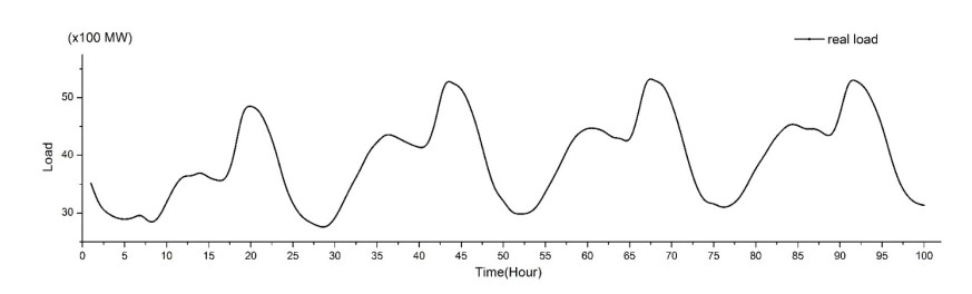
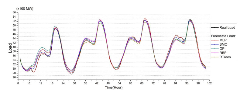
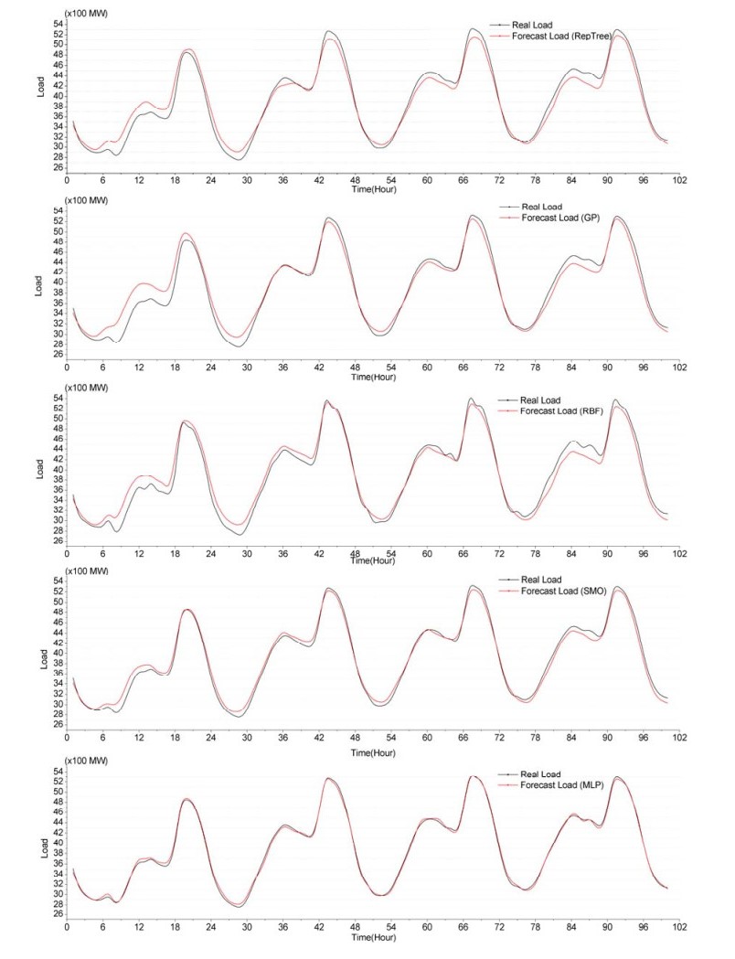
1. | Kei Hirose, Keigo Wada, Maiya Hori, Rin-ichiro Taniguchi, Event Effects Estimation on Electricity Demand Forecasting, 2020, 13, 1996-1073, 5839, 10.3390/en13215839 | |
2. | Mel Keytingan M. Shapi, Nor Azuana Ramli, Lilik J. Awalin, Energy consumption prediction by using machine learning for smart building: Case study in Malaysia, 2021, 5, 26661659, 100037, 10.1016/j.dibe.2020.100037 | |
3. | Davut Solyali, A Comparative Analysis of Machine Learning Approaches for Short-/Long-Term Electricity Load Forecasting in Cyprus, 2020, 12, 2071-1050, 3612, 10.3390/su12093612 | |
4. | Iwan Pahendra, Eva Darnila, Muhammad Sadli, Marzuki Sinambela, Wahyu Fuadi, 2019, Peak Load Forecasting Based on Long Short Term Memory, 978-1-7281-2930-3, 137, 10.1109/ICIMCIS48181.2019.8985197 | |
5. | S. Carcangiu, A. Fanni, P. A. Pegoraro, G. Sias, S. Sulis, Forecasting-Aided Monitoring for the Distribution System State Estimation, 2020, 2020, 1076-2787, 1, 10.1155/2020/4281219 | |
6. | Krishna Kumar, Ravindra Pratap Singh, Prashant Ranjan, Narendra Kumar, 2021, Chapter 65, 978-981-33-4603-1, 819, 10.1007/978-981-33-4604-8_65 | |
7. | Amine Khatib, Franck Dufrenois, Mohamed Hamlich, Denis Hamad, 2022, Chapter 4, 978-3-031-20489-0, 34, 10.1007/978-3-031-20490-6_4 | |
8. | Chafak Tarmanini, Nur Sarma, Cenk Gezegin, Okan Ozgonenel, Short term load forecasting based on ARIMA and ANN approaches, 2023, 9, 23524847, 550, 10.1016/j.egyr.2023.01.060 | |
9. | Agbassou Guenoupkati, Adekunle Akim Salami, Mawugno Koffi Kodjo, Kossi Nano, 2021, Short-Term Electricity Load Forecasting Using K-Means Clustering - Artificial Neural Networks Hybrid Model: Case Study Of Benin Electricity Community (CEB), 978-1-6654-4873-4, 01, 10.1109/HiTech53072.2021.9614236 | |
10. | Faisal Mehmood Butt, Lal Hussain, Syed Hassan Mujtaba Jafri, Haya Mesfer Alshahrani, Fahd N Al-Wesabi, Kashif Javed Lone, Elsayed M. Tag El Din, Mesfer Al Duhayyim, Intelligence based Accurate Medium and Long Term Load Forecasting System, 2022, 36, 0883-9514, 10.1080/08839514.2022.2088452 | |
11. | Aidos Satan, Ayagoz Khamzina, Damir Toktarbayev, Zhuldyz Sotsial, Ideyat Bapiyev, Nurkhat Zhakiyev, 2022, Comparative LSTM and SVM Machine Learning Approaches for Energy Consumption Prediction: Case Study in Akmola, 978-1-6654-6790-2, 1, 10.1109/SIST54437.2022.9945776 | |
12. | Giuliano Armano, Paolo Attilio Pegoraro, Assessing Feature Importance for Short-Term Prediction of Electricity Demand in Medium-Voltage Loads, 2022, 15, 1996-1073, 549, 10.3390/en15020549 | |
13. | Vira Shendryk, Yuliia Parfenenko, Sergii Tymchuk, Yevhen Kholiavka, Yaroslava Bielka, 2022, 2638, 0094-243X, 030004, 10.1063/5.0100123 | |
14. | Razak Olu-Ajayi, Hafiz Alaka, Ismail Sulaimon, Funlade Sunmola, Saheed Ajayi, Machine learning for energy performance prediction at the design stage of buildings, 2022, 66, 09730826, 12, 10.1016/j.esd.2021.11.002 | |
15. | Sivakavi Naga Venkata Bramareswara Rao, Venkata Pavan Kumar Yellapragada, Kottala Padma, Darsy John Pradeep, Challa Pradeep Reddy, Mohammad Amir, Shady S. Refaat, Day-Ahead Load Demand Forecasting in Urban Community Cluster Microgrids Using Machine Learning Methods, 2022, 15, 1996-1073, 6124, 10.3390/en15176124 | |
16. | Nishant Jha, Deepak Prashar, Mamoon Rashid, Sachin Kumar Gupta, R.K. Saket, Electricity load forecasting and feature extraction in smart grid using neural networks, 2021, 96, 00457906, 107479, 10.1016/j.compeleceng.2021.107479 | |
17. | Atif Maqbool Khan, Artur Wyrwa, A Survey of Quantitative Techniques in Electricity Consumption—A Global Perspective, 2024, 17, 1996-1073, 4910, 10.3390/en17194910 | |
18. | Mohammed Rashad Baker, Kamal H. Jihad, Hussein Al-Bayaty, Ahmed Ghareeb, Hessein Ali, Jun-Ki Choi, Qiancheng Sun, Uncertainty management in electricity demand forecasting with machine learning and ensemble learning: Case studies of COVID-19 in the US metropolitans, 2023, 123, 09521976, 106350, 10.1016/j.engappai.2023.106350 | |
19. | Paradhasaradhi Yeleswarpu, Rakesh Nayak, R. D. Patidar, 2024, Chapter 13, 978-3-031-48887-0, 151, 10.1007/978-3-031-48888-7_13 | |
20. | Sulagna Mahata, Piyush Harsh, Vineet Shekher, Comparative study of time-series forecasting models for wind power generation in Gujarat, India, 2024, 8, 27726711, 100511, 10.1016/j.prime.2024.100511 | |
21. | Waqar Waheed, Xu Qingshan, An efficient load forecasting technique by using Holt‐Winters and Prophet algorithms to mitigate the impact on power consumption in COVID‐19, 2024, 2516-8401, 10.1049/esi2.12132 | |
22. | Balarihun Mawtyllup, Bikramjit Goswami, 2024, Chapter 23, 978-981-99-4361-6, 243, 10.1007/978-981-99-4362-3_23 | |
23. | Xianan Huang, Wenjin Jiang, Xiaodong Yang, Zhenda Hu, Lin Liu, Xiazhe Tu, Chuangxin Guo, 2023, Electricity Load Combination Prediction Based on Fuzzy Clustering, 979-8-3503-4827-9, 944, 10.1109/CEEPE58418.2023.10165887 | |
24. | Oscar Villegas Mier, Anna Dittmann, Wiebke Herzberg, Holger Ruf, Elke Lorenz, Michael Schmidt, Rainer Gasper, Predictive Control of a Real Residential Heating System with Short-Term Solar Power Forecast, 2023, 16, 1996-1073, 6980, 10.3390/en16196980 | |
25. | E. U. Archibong-Eso, A. Archibong-Eso, J. D. Enyia, 2023, Machine Learning Models for Energy Prediction in a Low Carbon Building, 10.2118/217259-MS | |
26. | Muhammad Anan, Khalid Kanaan, Driss Benhaddou, Nidal Nasser, Basheer Qolomany, Hanaa Talei, Ahmad Sawalmeh, Occupant-Aware Energy Consumption Prediction in Smart Buildings Using a LSTM Model and Time Series Data, 2024, 17, 1996-1073, 6451, 10.3390/en17246451 | |
27. | Elhabyb Khaoula, Baina Amine, Bellafkih Mostafa, 2025, Chapter 14, 978-3-031-71913-4, 117, 10.1007/978-3-031-71914-1_14 | |
28. | Lucas de Azevedo Takara, Luis Fernando Rodrigues Agottani, Cesar Vinicius Züge, Wendel Rafael de Souza Chaves, Leandro dos Santos Coelho, Viviana Cocco Mariani, 2024, Deep Learning-Based Probabilistic Forecasting of Household Energy Consumption in Smart Grids, 979-8-3503-9042-1, 1, 10.1109/ISGTEUROPE62998.2024.10863218 | |
29. | Rahul R. Patil, Mukesh Kumar Gupta, Kishor V. Bhadane, 2025, Electrical Energy Forecasting of Industrial Feeder from Rural Area Using Different Regression Techniques, 979-8-3503-5561-1, 1, 10.1109/ICAET63349.2025.10932244 | |
30. | Ashutosh Shukla, Rupendra Kumar Pachauri, 2025, 9781394249435, 347, 10.1002/9781394249466.ch13 |
SMO | RBF | GP | RepTree | MLP | |
MAPE | 2.02 | 3.14 | 3.29 | 3.01 | 0.97 |
MAE | 7519 | 11663 | 12087 | 11464 | 3654 |
MSE | 779570 | 1914368 | 2481405 | 1890943 | 180647 |