The health status (HS) of children is influenced by a variety of factors, including physical fitness (PF) or social and environmental characteristics. We present a 4-year longitudinal study carried out with 263 primary school children. PF was assessed yearly using the German Motor Performance Test 6–18. Demographic data, leisure time behavior and socioeconomic factors were collected using questionnaires for children and parents. Based on parents' ratings in year 4, children were categorized as either “very good health status” (VGHS) or “good health status or below” (GHSB). Children with VGHS (73%) showed a larger improvement of global PF (p < 0.001), a significantly higher proportion of being/playing outside (p < 0.001), significantly lower proportions of overweight (p < 0.001), of media availability in the bedroom (p = 0.011) and of daily media consumption > 2 h (p = 0.033) compared to children with GHSB. Regarding socio-economic factors, children with VGHS revealed significantly fewer parents with lower education (p = 0.002), lower physical activity levels (p = 0.030) and lower migration background (p < 0.001). Physical fitness (p = 0.019) and outdoors exercising (p = 0.050) were the only variables to provide significantly higher chances of perceiving one's own health as very good when tested within a complex model including all the variables studied in this work. Considering the little focus on PF in the current Austrian physical education curriculum and the favorable environmental features of the Tyrolean region, more emphasis should be given to promoting didactical and pedagogical approaches that allow schoolers to be active in the nature.
Citation: Gerhard Ruedl, Armando Cocca, Katharina C. Wirnitzer, Derrick Tanous, Clemens Drenowatz, Martin Niedermeier. Primary school children's health and its association with physical fitness development and health-related factors[J]. AIMS Public Health, 2024, 11(1): 1-18. doi: 10.3934/publichealth.2024001
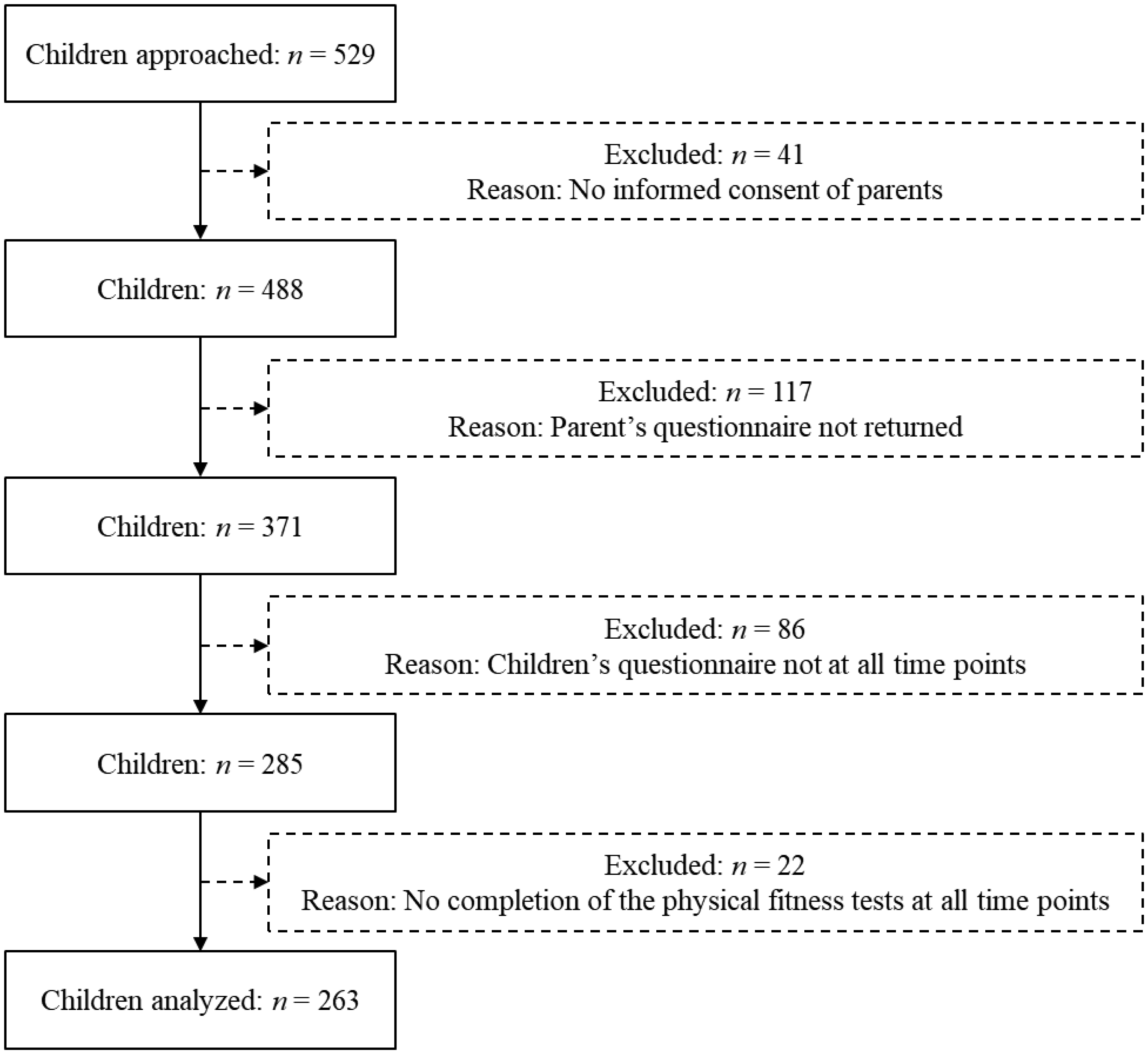
The health status (HS) of children is influenced by a variety of factors, including physical fitness (PF) or social and environmental characteristics. We present a 4-year longitudinal study carried out with 263 primary school children. PF was assessed yearly using the German Motor Performance Test 6–18. Demographic data, leisure time behavior and socioeconomic factors were collected using questionnaires for children and parents. Based on parents' ratings in year 4, children were categorized as either “very good health status” (VGHS) or “good health status or below” (GHSB). Children with VGHS (73%) showed a larger improvement of global PF (p < 0.001), a significantly higher proportion of being/playing outside (p < 0.001), significantly lower proportions of overweight (p < 0.001), of media availability in the bedroom (p = 0.011) and of daily media consumption > 2 h (p = 0.033) compared to children with GHSB. Regarding socio-economic factors, children with VGHS revealed significantly fewer parents with lower education (p = 0.002), lower physical activity levels (p = 0.030) and lower migration background (p < 0.001). Physical fitness (p = 0.019) and outdoors exercising (p = 0.050) were the only variables to provide significantly higher chances of perceiving one's own health as very good when tested within a complex model including all the variables studied in this work. Considering the little focus on PF in the current Austrian physical education curriculum and the favorable environmental features of the Tyrolean region, more emphasis should be given to promoting didactical and pedagogical approaches that allow schoolers to be active in the nature.

| [1] | World Health OrganizationHealthy grow and development (2023). Available from: https://www.who.int/teams/maternal-newborn-child-adolescent-health-and-ageing/child-health/healthy-growth-and-development |
| [2] |
Carreras M, Puig G, Sanchez-Perez I, et al. (2020) Morbidity and self-perception of health, two different approaches to health status. Gac Sanit 34: 601-607. https://doi.org/10.1016/j.gaceta.2019.04.005 
|
| [3] |
Werneck AO, Silva DR, Agostinete RR, et al. (2018) Relationship of parental and adolescents' screen time to self-rated health: a structural equation modeling. Health Educ Behav 45: 764-771. https://doi.org/10.1177/1090198118757825
|
| [4] |
Zhang T, Lu G, Wu XY (2020) Associations between physical activity, sedentary behavior and self-rated health among the general population of children and adolescents: A systematic review and meta-analysis. BMC Public health 20: 1343. https://doi.org/10.1186/s12889-020-09447-1
|
| [5] |
Pascual SC, Casajús Mallén JA, González Gross M (2020) Adherence factors related to exercise prescriptions in healthcare settings: A review of the scientific literature. Res Q Exerc Sport 93: 16-25. https://doi.org/10.1080/02701367.2020.1788699
|
| [6] |
Burke S, Utley A, Belchamber C, McDowall L (2020) Physical activity in hospice care: A social ecological perspective to inform policy and practice. Res Q Exerc Sport 91: 500-513. https://doi.org/10.1080/02701367.2019.1687808
|
| [7] |
Da Silva AO, Diniz PRB, Santons M, et al. (2019) Health self-perception and its association with physical activity and nutritional status in adolescents. J Pediatr 95: 458-465. https://doi.org/10.1016/j.jped.2018.05.007
|
| [8] |
Moral Garcia JE, Agraso Lopez AD, Ramos Morcillo AJ, et al. (2020) The influence of physical activity, diet, weight status and substance abuse on students' self-perceived health. Int J Environ Res Public Health 17: 1387. https://doi.org/10.3390/ijerph17041387
|
| [9] |
Rittsteiger L, Hinz T, Oriwol D, et al. (2022) Changes of self-rated health status, overweight and physical activity during childhood and adolescence-the ratchet effect of high parental socioeconomic status. Front Sports Act Living 4: 781394. https://doi.org/10.3389/fspor.2022.781394
|
| [10] |
Brodersen K, Hammami N, Katapally TR (2023) Is excessive smartphone use associated with weight status and self-rated health among youth? A smart platform study. BMC Public Health 23: 234. https://do.org/10.1186/s12889-023-15037-8
|
| [11] |
Mintjens S, Menting MD, Daams JG, et al. (2018) Cardiorespiratory fitness in childhood and adolescence affects future cardiovascular risk factors: A systematic review of longitudinal studies. Sports Med 48: 2577-2605. https://doi.org/10.1007/s40279-018-0974-5
|
| [12] |
Tomkinson GR, Carver KD, Atkinson F, et al. (2018) European normative values for physical fitness in children and adolescents aged 9–17 years: Results from 2 779 165 Eurofit performances representing 30 countries. Br J Sports Med 52: 1445-14563. https://doi.org/10.1136/bjsports-2017-098253
|
| [13] |
García-Hermoso A, Ramírez-Campillo R, Izquierdo M (2019) Is muscular fitness associated with future health benefits in children and adolescents? A systematic review and meta-analysis of longitudinal studies. Sports Med 49: 1079-1094. https://doi.org/10.1007/s40279-019-01098-6
|
| [14] |
Ortega FB, Silventoinen K, Tynelius P, et al. (2012) Muscular strength in male adolescents and premature death: Cohort study of one million participants. BMJ 20: e7279. https://doi.org/10.1136/bmj.e7279
|
| [15] |
Högström G, Ohlsson H, Crump C, et al. (2019) Aerobic fitness in late adolescence and the risk of cancer and cancer-associated mortality in adulthood: A prospective nationwide study of 1.2 million Swedish men. Cancer Epidemiol 59: 58-63. https://doi.org/10.1016/j.canep.2019.01.012
|
| [16] |
Krause L, Mauz E (2018) Subjective, physical and mental health of children and adolescents in Thuringia: Representative results ealth Thuringia state module in KiGGS wave. Bundesgesundheitsblatt Gesundheitsforschung Gesundheitsschutz 61: 845-856. https://doi.org/10.1007/s00103-018-2753-8
|
| [17] |
Elissa K, Bratt EL, Axelsson ÅB, et al. (2020) Self-perceived health status and sense of coherence in children with type 1 diabetes in the west bank, Palestine. J Transcult Nurs 31: 153-161. https://doi.org/10.1177/1043659619854509
|
| [18] |
Husu P, Vaha-Ypya H, Vasankari T (2016) Objectively measured sedentary behavior and physical activity of Finnish 7- to 14-year-old children- association with perceived health status: A cross-sectional study. BMC Public Health 16: 338. https://doi.org/10.1186/s12889-016-3006-0
|
| [19] |
Padilla-Moledo C, Fernández-Santos JDR, Izquierdo-Gómez R, et al. (2020) Physical fitness and self-rated health in children and adolescents: Cross-sectional and longitudinal study. Int J Environ Res Public Health 17: 2413. https://doi.org/10.3390/ijerph17072413
|
| [20] |
Hanssen-Doose A, Kunina-Habenicht O, Oriwol D, et al. (2021) Predictive value of physical fitness on self-rated health: A longitudinal study. Scand J Me Sci Sports 31: 56-64. https://doi.org/10.1111/sms.13841
|
| [21] |
Kromeyer-Hauschild K, Wabitsch M, Kunze D, et al. (2001) Perzentile für den Body-Mass-Index für das Kindes- und Jugendalter unter Heranziehung verschiedener deutscher Stichproben. Monatsschrift Kinderheilkunde 149: 807-818. https://doi.org/10.1007/s001120170107
|
| [22] | Bös K, Schlenker L, Büsch D, et al. (2009) Deutscher Motorik Test 6–18 (DMT 6–18). German motor performance test (DMT 6–18) . Berlin, GER: Czwalina 6-18. |
| [23] |
Utesch T, Dreiskamper D, Strauss B, et al. (2018) The development of the physical fitness construct across childhood. Scand J Med Sci Sports 28: 212-219. https://doi.org/10.1111/sms.12889
|
| [24] |
Ruedl G, Ewald P, Niedermeier M, et al. (2019) Long-term effect of migration background on the development of physical fitness among primary school children. Scand J Med Sci Sports 29: 124-131. https://doi.org/10.1111/sms.13316
|
| [25] | UNESCO Institute for StatisticsInternational Standard Classification of Education (ISCED) (2012). Available from: http://uis.unesco.org/sites/default/files/documents/international-standard-classification-of-education-isced-2011-en.pdf |
| [26] |
Ruedl G, Niedermeier M, Wimmer L, et al. (2021) Impact of parental education and physical activity on the long-term development of the physical fitness of primary school children: An observational study. Int J Environ Res Public Health 18: 8736. https://doi.org/10.3390/ijerph18168736
|
| [27] |
Ruedl G, Niedermeier M, Posch M, et al. (2022) Association of modifiable factors with the development of physical fitness of Austrian primary school children: A 4-year longitudinal study. J Sports Sciences 40: 920-927. https://doi.org/10.1080/02640414.2022.2038874
|
| [28] |
Burchatz A, Oriwol D, Kolb S, et al. (2021) Comparison of self-reported device-based, measured physical activity among children in Germany. BMC Public Health 21: 1081. https://doi.org/10.1186/s12889-021-11114-y
|
| [29] | Cohen J (1988) Statistical Power Analysis for the Behavioral Sciences. New York, USA: Lawrence Erlbaum Associates 20-27. |
| [30] | Field A (2018) Discovering Statistics Using IBM SPSS Statistics. Thousand Oaks, CA: SAGE Publications Ltd 95-134. |
| [31] |
Cocca A, Espino Verdugo F, Rodenas Cuenca L, et al. (2020) Effect of a game-based physical education program on physical fitness and mental health in elementary school children. Int J Environ Res Public Health 17: 4883. https://doi.org/10.3390/ijerph17134883
|
| [32] |
Cocca A, Carbajal Baca J, Hernandez Cruz G, et al. (2020) Does a multiple-sport intervention based on the TgfU model for physical education increase physical fitness in primary school children?. Int J Environ Res Public Health 17: 5532. https://doi.org/10.3390/ijerph17155532
|
| [33] | Peralta M, Henriques-Neto D, Gouveia ER, et al. (2020) Promoting health-related cardiorespiratory fitness in physical education: A systematic review. PloS One 15: 0237019. https://doi.org/10.1371/journal.pone.0237019 |
| [34] |
Kantomaa MT, Tammelin T, Ebeling H, et al. (2015) High levels of physical activity and cardiorespiratory fitness are associated with good self-rated health in adolescents. J Phys Act Health 12: 266-272. https://doi.org/10.1123/jpah.2013-0062
|
| [35] |
Eriksen L, Curtis T, Gronbaek M, et al. (2013) The association between physical activity, cardiorespiratory fitness and self-rated health. Prev Med 57: 900-902. https://doi.org/10.1016/j.ypmed.2013.09.024
|
| [36] |
Herman KM, Hopman WM, Sabiston CM (2015) Physical activity, screen time and self-rated health and mental health in Canadian adolescents. Prev Med 73: 112-116. https://doi.org/10.1016/j.ypmed.2015.01.030
|
| [37] |
Breidablik HJ, Meland E, Lydersen S (2009) Self-rated health during adolescence: Stability and predictors of change (Young-HUNT study, Norway). Eur J Public Health 19: 73-78. https://doi.org/10.1093/eurpub/ckn111
|
| [38] |
Krause L, Lampert T (2015) Relation between overweight/obesity and self-rated health among adolescents in Germany. Do socio-economic status and type of school have an impact on that relation?. Int J Environ Res Public Health 12: 2262-2276. https://doi.org/10.3390/ijerph120202262
|
| [39] |
Mbogori T, Arthur TM (2019) Perception of body weight status is associated with the health and food intake behaviors of adolescents in the United States. Am J Lifestyle Med 15: 347-355. https://doi.org/10.1177/1559827619834507
|
| [40] |
Meland E, Breidablik HJ, Thuen F, et al. (2021) How body concerns, body mass, self-rated health and self-esteem are mutually impacted in early adolescence: A longitudinal cohort study. BMC Public Health 21: 496. https://doi.org/10.1186/s12889-021-10553-x
|
| [41] |
Matin N, Kelishadi R, Heshmat R, et al. (2017) Joint association of screen time and physical activity on self-rated health and life satisfaction in children and adolescents: The CASPIAN-IV study. Int Health 9: 58-68. https://doi.org/10.1093/inthealth/ihw044
|
| [42] |
Greier K, Drenowatz C, Ruedl G, et al. (2019) Association between daily TV time and fitness in 6- to 14-year old Austrian youth. Transl Pediatr 8: 371-377. https://doi.org/10.21037/tp.2019.03.03
|
| [43] |
Vermeiren AP, Willeboordse M, Oosterhoff M, et al. (2018) Socioeconomic multi-domain health inequalities in Dutch primary school children. Eur J Public Health 28: 610-616. https://doi.org/10.1093/eurpub/cky055
|
| [44] |
Okamoto S (2021) Parental socioeconomic status and adolescent health in Japan. Sci Rep 11: 12089. https://doi.org/10.1038/s41598-021-91715-0
|
| [45] |
Kerr J, Marshall S, Godbole S, et al. (2012) The relationship between outdoor activity and health in older adults using GPS. Int J Environ Res Public Health 9: 4615-4625. https://doi.org/10.3390/ijerph9124615
|
| [46] |
Coventry PA, Brown JE, Pervin J, et al. (2021) Nature-based outdoor activities for mental and physical health: Systematic review and meta-analysis. SSM Popul Health 16: 100934. https://doi.org/10.1016/j.ssmph.2021.100934
|
| [47] |
Sando OJ (2019) The outdoor environment and children's health: A multilevel approach. Int J Play 8: 39-52. https://doi.org/10.1080/21594937.2019.1580336
|
| [48] |
Pasanen TP, Tyrväinen L, Korpela KM (2014) The relationship between perceived health and physical activity indoors, outdoors in built environments, and outdoors in nature. Appl Psychol Health Well Being 6: 324-346. https://doi.org/10.1111/aphw.12031
|
| [49] |
Stodden DF, Goodway JD, Langendorfer SJ, et al. (2008) A developmental perspective on the role of motor skill competence in physical activity: An emergent relationship. Quest 60: 290-306. https://doi.org/10.1080/00336297.2008.10483582
|
| [50] | (2018) World Health OrganizationAustria physical activity factsheet 2018. Geneva: WHO. Available from: https://www.euro.who.int/__data/assets/pdf_file/0009/382338/austria-eng.pdf. |
| [51] |
Pouline T, Ludwig J, Hiemisch A, et al. (2019) Media use of mothers, media use of children, and parent–child interaction are related to behavioral difficulties and strengths of children. Int J Environ Res Public Health 16: 4651. https://doi.org/10.3390/ijerph16234651
|
Figures(1) / Tables(4)

Gerhard Ruedl, Armando Cocca, Katharina C. Wirnitzer, Derrick Tanous, Clemens Drenowatz, Martin Niedermeier. Primary school children's health and its association with physical fitness development and health-related factors[J]. AIMS Public Health, 2024, 11(1): 1-18. doi: 10.3934/publichealth.2024001


 DownLoad: