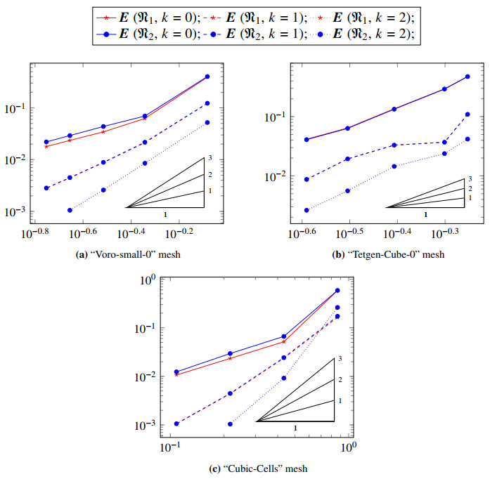
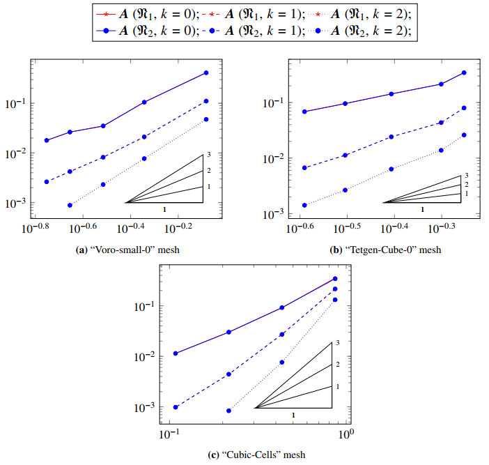
Two numerical schemes are proposed and investigated for the Yang–Mills equations, which can be seen as a nonlinear generalisation of the Maxwell equations set on Lie algebra-valued functions, with similarities to certain formulations of General Relativity. Both schemes are built on the Discrete de Rham (DDR) method, and inherit from its main features: an arbitrary order of accuracy, and applicability to generic polyhedral meshes. They make use of the complex property of the DDR, together with a Lagrange-multiplier approach, to preserve, at the discrete level, a nonlinear constraint associated with the Yang–Mills equations. We also show that the schemes satisfy a discrete energy dissipation (the dissipation coming solely from the implicit time stepping). Issues around the practical implementations of the schemes are discussed; in particular, the assembly of the local contributions in a way that minimises the price we pay in dealing with nonlinear terms, in conjunction with the tensorisation coming from the Lie algebra. Numerical tests are provided using a manufactured solution, and show that both schemes display a convergence in $ L^2 $-norm of the potential and electrical fields in $ \mathcal O(h^{k+1}) $ (provided that the time step is of that order), where $ k $ is the polynomial degree chosen for the DDR complex. We also numerically demonstrate the preservation of the constraint.
Citation: Jérôme Droniou, Jia Jia Qian. Two arbitrary-order constraint-preserving schemes for the Yang–Mills equations on polyhedral meshes[J]. Mathematics in Engineering, 2024, 6(3): 468-493. doi: 10.3934/mine.2024019
Two numerical schemes are proposed and investigated for the Yang–Mills equations, which can be seen as a nonlinear generalisation of the Maxwell equations set on Lie algebra-valued functions, with similarities to certain formulations of General Relativity. Both schemes are built on the Discrete de Rham (DDR) method, and inherit from its main features: an arbitrary order of accuracy, and applicability to generic polyhedral meshes. They make use of the complex property of the DDR, together with a Lagrange-multiplier approach, to preserve, at the discrete level, a nonlinear constraint associated with the Yang–Mills equations. We also show that the schemes satisfy a discrete energy dissipation (the dissipation coming solely from the implicit time stepping). Issues around the practical implementations of the schemes are discussed; in particular, the assembly of the local contributions in a way that minimises the price we pay in dealing with nonlinear terms, in conjunction with the tensorisation coming from the Lie algebra. Numerical tests are provided using a manufactured solution, and show that both schemes display a convergence in $ L^2 $-norm of the potential and electrical fields in $ \mathcal O(h^{k+1}) $ (provided that the time step is of that order), where $ k $ is the polynomial degree chosen for the DDR complex. We also numerically demonstrate the preservation of the constraint.

| [1] |
D. A. Di Pietro, J. Droniou, Homological- and analytical-preserving serendipity framework for polytopal complexes, with application to the DDR method, ESAIM: M2AN, 57 (2023), 191–225. https://doi.org/10.1051/m2an/2022067 doi: 10.1051/m2an/2022067

|
| [2] |
J. Droniou, T. A. Oliynyk, J. J. Qian, A polyhedral discrete de rham numerical scheme for the Yang–Mills equations, J. Comput. Phys., 478 (2023), 111955. https://doi.org/10.1016/j.jcp.2023.111955 doi: 10.1016/j.jcp.2023.111955
|
| [3] |
D. N. Arnold, R. S. Falk, R. Winther, Finite element exterior calculus, homological techniques, and applications, Acta Numer., 15 (2006), 1–155. https://doi.org/10.1017/S0962492906210018 doi: 10.1017/S0962492906210018
|
| [4] | D. Arnold, Finite element exterior calculus, Society for Industrial and Applied Mathematics, 2018. https://doi.org/10.1137/1.9781611975543 |
| [5] |
D. N. Arnold, R. S. Falk, R. Winther, Finite element exterior calculus: from Hodge theory to numerical stability, Bull. Amer. Math. Soc., 47 (2010), 281–354. https://doi.org/10.1090/S0273-0979-10-01278-4 doi: 10.1090/S0273-0979-10-01278-4
|
| [6] |
A. Gillette, K. Hu, S. Zhang, Nonstandard finite element de Rham complexes on cubical meshes, Bit Numer. Math., 60 (2020), 373–409. https://doi.org/10.1007/s10543-019-00779-y doi: 10.1007/s10543-019-00779-y
|
| [7] | D. Arnold, K. Hu, Complexes from complexes, Found. Comput. Math., 21 (2021), 1739–1774. https://doi.org/10.1007/s10208-021-09498-9 |
| [8] | D. Di Pietro, M. Hanot, A discrete three-dimensional{\rm{div}}div complex on polyhedral meshes with application to a mixed formulation of the biharmonic problem, arXiv, 2023. https://doi.org/10.48550/arXiv.2305.05729 |
| [9] |
L. Beirão da Veiga, F. Brezzi, L. D. Marini, A. Russo, H(div) and H(curl)-conforming VEM, Numer. Math., 133 (2016), 303–332. https://doi.org/10.1007/s00211-015-0746-1 doi: 10.1007/s00211-015-0746-1
|
| [10] |
L. Beirão da Veiga, F. Brezzi, F. Dassi, L. D. Marini, A. Russo, A family of three-dimensional virtual elements with applications to magnetostatics, SIAM J. Numer. Anal., 56 (2018), 2940–2962. https://doi.org/10.1137/18M1169886 doi: 10.1137/18M1169886
|
| [11] |
D. A. Di Pietro, J. Droniou, F. Rapetti, Fully discrete polynomial de Rham sequences of arbitrary degree on polygons and polyhedra, Math. Models Methods Appl. Sci., 30 (2020), 1809–1855. https://doi.org/10.1142/S0218202520500372 doi: 10.1142/S0218202520500372
|
| [12] |
D. A. Di Pietro, J. Droniou, An arbitrary-order discrete de Rham complex on polyhedral meshes: exactness, Poincaré inequalities, and consistency, Found. Comput. Math., 23 (2023), 85–164. https://doi.org/10.1007/s10208-021-09542-8 doi: 10.1007/s10208-021-09542-8
|
| [13] |
D. A. Di Pietro, J. Droniou, An arbitrary-order method for magnetostatics on polyhedral meshes based on a discrete de Rham sequence, J. Comput. Phys., 429 (2021), 109991. https://doi.org/10.1016/j.jcp.2020.109991 doi: 10.1016/j.jcp.2020.109991
|
| [14] | D. A. Di Pietro, J. Droniou, A discrete de Rham method for the Reissner-Mindlin plate bending problem on polygonal meshes, arXiv, 2021. https://doi.org/10.48550/arXiv.2105.11773 |
| [15] |
D. A. Di Pietro, J. Droniou, A fully discrete plates complex on polygonal meshes with application to the Kirchhoff–Love problem, Math. Comp., 92 (2023), 51–77. https://doi.org/10.1090/mcom/3765 doi: 10.1090/mcom/3765
|
| [16] |
L. Chen, X. Huang, Decoupling of mixed methods based on generalized Helmholtz decompositions, SIAM J. Numer. Anal., 56 (2018), 2796–2825. https://doi.org/10.1137/17M1145872 doi: 10.1137/17M1145872
|
| [17] |
L. Chen, X. Huang, Finite elements for{\rm{div}}- and{\rm{div}}div-conforming symmetric tensors in arbitrary dimension, SIAM J. Numer. Anal., 60 (2022), 1932–1961. https://doi.org/10.1137/21M1433708 doi: 10.1137/21M1433708
|
| [18] |
L. Beirão da Veiga, F. Dassi, D. A. Di Pietro, J. Droniou, Arbitrary-order pressure-robust DDR and VEM methods for the Stokes problem on polyhedral meshes, Comput. Meth. Appl. Mech. Eng., 397 (2022), 115061. https://doi.org/10.1016/j.cma.2022.115061 doi: 10.1016/j.cma.2022.115061
|
| [19] |
L. Beirão da Veiga, F. Dassi, G. Vacca, The stokes complex for virtual elements in three dimensions, Math. Models Methods Appl. Sci., 30 (2020), 477–512. https://doi.org/10.1142/S0218202520500128 doi: 10.1142/S0218202520500128
|
| [20] |
S. H. Christiansen, R. Winther, On constraint preservation in numerical simulations of Yang–Mills equations, SIAM J. Sci. Comput., 28 (2006), 75–101. https://doi.org/10.1137/040616887 doi: 10.1137/040616887
|
| [21] |
Y. Berchenko-Kogan, A. Stern, Charge-conserving hybrid methods for the Yang–Mills equations, SMAI J. Comput. Math., 7 (2021), 97–119. https://doi.org/10.5802/smai-jcm.73 doi: 10.5802/smai-jcm.73
|
| [22] |
D. Alic, C. Bona-Casas, C. Bona, L. Rezzolla, C. Palenzuela, Conformal and covariant formulation of the Z4 system with constraint-violation damping, Phys. Rev. D, 85 (2012), 064040. https://doi.org/10.1103/PhysRevD.85.064040 doi: 10.1103/PhysRevD.85.064040
|
| [23] |
O. Brodbeck, S. Frittelli, P. Hübner, O. A. Reula, Einstein's equations with asymptotically stable constraint propagation, J. Math. Phys., 40 (1999), 909–923. https://doi.org/10.1063/1.532694 doi: 10.1063/1.532694
|
| [24] |
J. Frauendiener, T. Vogel, Algebraic stability analysis of constraint propagation, Class. Quantum Grav., 22 (2005), 1769. https://doi.org/10.1088/0264-9381/22/9/019 doi: 10.1088/0264-9381/22/9/019
|
| [25] |
C. Gundlach, G. Calabrese, I. Hinder, J. M. Martín-García, Constraint damping in the Z4 formulation and harmonic gauge, Class. Quantum Grav., 22 (2005), 3767. https://doi.org/10.1088/0264-9381/22/17/025 doi: 10.1088/0264-9381/22/17/025
|
| [26] |
H. Friedrich, Hyperbolic reductions for Einstein's equations, Class. Quantum Grav., 13 (1996), 1451. https://doi.org/10.1088/0264-9381/13/6/014 doi: 10.1088/0264-9381/13/6/014
|
| [27] |
A. Anderson, Y. Choquet-Bruhat, J. W. York Jr., Einstein-Bianchi hyperbolic system for general relativity, Topol. Methods Nonlinear Anal., 10 (1997), 353–373. https://doi.org/10.12775/TMNA.1997.037 doi: 10.12775/TMNA.1997.037
|
| [28] | D. A. Di Pietro, J. Droniou, The Hybrid High-Order method for polytopal meshes: design, analysis, and applications, Springer Cham, 2020. https://doi.org/10.1007/978-3-030-37203-3 |
| [29] | F. Bonaldi, D. A. Di Pietro, J. Droniou, K. Hu, An exterior calculus framework for polytopal methods, arXiv, 2023. https://doi.org/10.48550/arXiv.2303.11093 |
| [30] |
D. A. Di Pietro, J. Droniou, S. Pitassi, Cohomology of the discrete de Rham complex on domains of general topology, Calcolo, 60 (2023), 32. https://doi.org/10.1007/s10092-023-00523-7 doi: 10.1007/s10092-023-00523-7
|
| [31] |
D. A. Di Pietro, J. Droniou, A third Strang lemma and an Aubin-Nitsche trick for schemes in fully discrete formulationn, Calcolo, 55 (2018), 40. https://doi.org/10.1007/s10092-018-0282-3 doi: 10.1007/s10092-018-0282-3
|
Figures(2) / Tables(3)

Jérôme Droniou, Jia Jia Qian. Two arbitrary-order constraint-preserving schemes for the Yang–Mills equations on polyhedral meshes[J]. Mathematics in Engineering, 2024, 6(3): 468-493. doi: 10.3934/mine.2024019


 DownLoad: