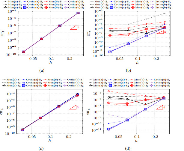
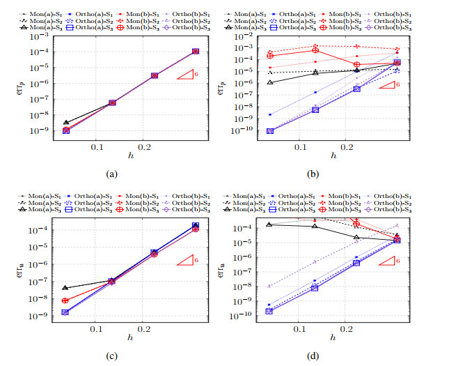
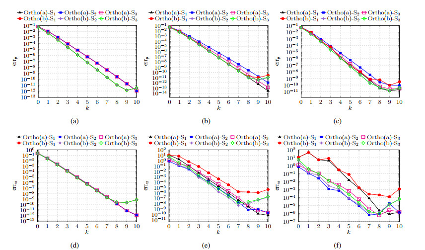
In this paper, we discuss the accuracy and the robustness of the mixed Virtual Element Methods when dealing with highly anisotropic diffusion problems. In particular, we analyze the performance of different approaches which are characterized by different sets of both boundary and internal degrees of freedom in the presence of a strong anisotropy of the diffusion tensor with constant or variable coefficients. A new definition of the boundary degrees of freedom is also proposed and tested.
Citation: Stefano Berrone, Stefano Scialò, Gioana Teora. The mixed virtual element discretization for highly-anisotropic problems: the role of the boundary degrees of freedom[J]. Mathematics in Engineering, 2023, 5(6): 1-32. doi: 10.3934/mine.2023099
In this paper, we discuss the accuracy and the robustness of the mixed Virtual Element Methods when dealing with highly anisotropic diffusion problems. In particular, we analyze the performance of different approaches which are characterized by different sets of both boundary and internal degrees of freedom in the presence of a strong anisotropy of the diffusion tensor with constant or variable coefficients. A new definition of the boundary degrees of freedom is also proposed and tested.

| [1] | Finite Volume Schemes on general grids, for anisotropic and heterogeneous diffusion problems. Available from: https://www.i2m.univ-amu.fr//fvca5//benchmark//Meshes//#mesh4. |
| [2] |
B. Andreianov, F. Boyer, F. Hubert, Discrete duality finite volume schemes for Leray-Lions type elliptic problems on general 2D meshes, Numer. Meth. Part. Differ. Equ., 23 (2007), 145–195. https://doi.org/10.1002/num.20170 doi: 10.1002/num.20170

|
| [3] |
O. Angelini, C. Chavant, E. Chénier, R. Eymard, A finite volume scheme for diffusion problems on general meshes applying monotony constraints, SIAM J. Numer. Anal., 47 (2010), 4193–4213. https://doi.org/10.1137/080732183 doi: 10.1137/080732183
|
| [4] | I. Babuška, M. Suri, On locking and robustness in the finite element method, SIAM J. Numer. Anal., 29 (1992), 1261–1293. |
| [5] |
F. Bassi, L. Botti, A. Colombo, D. A. Di Pietro, P. Tesini, On the flexibility of agglomeration based physical space discontinuous Galerkin discretizations, J. Comput. Phys., 231 (2012), 45–65. https://doi.org/10.1016/j.jcp.2011.08.018 doi: 10.1016/j.jcp.2011.08.018
|
| [6] |
L. Beirão da Veiga, F. Brezzi, L. D. Marini, A. Russo, Virtual element method for general second-order elliptic problems on polygonal meshes, Math. Mod. Meth. Appl. Sci., 26 (2016), 729–750. https://doi.org/10.1142/S0218202516500160 doi: 10.1142/S0218202516500160
|
| [7] |
L. Beirão da Veiga, F. Brezzi, A. Cangiani, G. Manzini, L. D. Marini, A. Russo, Basic principles of virtual element methods, Math. Mod. Meth. Appl. Sci., 23 (2013), 199–214. https://doi.org/10.1142/S0218202512500492 doi: 10.1142/S0218202512500492
|
| [8] |
L. Beirão da Veiga, F. Brezzi, L. D. Marini, A. Russo, Mixed virtual element methods for general second order elliptic problems on polygonal meshes, ESAIM: M2AN, 50 (2016), 727–747. https://doi.org/10.1051/m2an/2015067 doi: 10.1051/m2an/2015067
|
| [9] | L. Beirão da Veiga, F. Brezzi, L. D. Marini, A. Russo, Virtual element implementation for general elliptic equations, In: G. Barrenechea, F. Brezzi, A. Cangiani, E. Georgoulis, Building bridges: connections and challenges in modern approaches to numerical partial differential equations, Lecture Notes in Computational Science and Engineering, Cham: Springer, 114 (2016), 39–71. https://doi.org/10.1007/978-3-319-41640-3_2 |
| [10] |
L. Beirão da Veiga, F. Dassi, A. Russo, High-order Virtual Element Method on polyhedral meshes, Comput. Math. Appl., 74 (2017), 1110–1122. https://doi.org/10.1016/j.camwa.2017.03.021 doi: 10.1016/j.camwa.2017.03.021
|
| [11] |
S. Berrone, A. Borio, Orthogonal polynomials in badly shaped polygonal elements for the Virtual Element Method, Finite Elem. Anal. Des., 129 (2017), 14–31. https://doi.org/10.1016/j.finel.2017.01.006 doi: 10.1016/j.finel.2017.01.006
|
| [12] | S. Berrone, A. Borio, F. Marcon, Lowest order stabilization free Virtual Element Method for the 2D Poisson equation, arXiv, 2023. https://doi.org/10.48550/arXiv.2103.16896 |
| [13] |
S. Berrone, G. Teora, F. Vicini, Improving high-order VEM stability on badly-shaped elements, Math. Comput. Simul., 216 (2024), 367–385. https://doi.org/10.1016/j.matcom.2023.10.003 doi: 10.1016/j.matcom.2023.10.003
|
| [14] | S. Berrone, S. Scialó, G. Teora, Orthogonal polynomial bases in the Mixed Virtual Element Method, arXiv, 2023. https://doi.org/10.48550/arXiv.2304.14755 |
| [15] |
F. Brezzi, R. S. Falk, L. D. Marini, Basic principles of mixed Virtual Element Methods, ESAIM: Math. Modell. Numer. Anal., 48 (2014), 1227–1240. https://doi.org/10.1051/m2an/2013138 doi: 10.1051/m2an/2013138
|
| [16] |
F. Dassi, L. Mascotto, Exploring high-order three dimensional virtual elements: bases and stabilizations, Comput. Math. Appl., 75 (2018), 3379–3401. https://doi.org/10.1016/j.camwa.2018.02.005 doi: 10.1016/j.camwa.2018.02.005
|
| [17] |
G. Giorgiani, H. Bufferand, F. Schwander, E. Serre, P. Tamain, A high-order non field-aligned approach for the discretization of strongly anisotropic diffusion operators in magnetic fusion, Comput. Phys. Commun., 254 (2020), 107375. https://doi.org/10.1016/j.cpc.2020.107375 doi: 10.1016/j.cpc.2020.107375
|
| [18] |
D. Green, X. Hu, J. Lore, L. Mu, M. L. Stowell, An efficient high-order numerical solver for diffusion equations with strong anisotropy, Comput. Phys. Commun., 276 (2022), 108333. https://doi.org/10.1016/j.cpc.2022.108333 doi: 10.1016/j.cpc.2022.108333
|
| [19] |
V. Havu, J. Pitkäranta, An analysis of finite element locking in a parameter dependent model problem, Numer. Math., 89 (2001), 691–714. https://doi.org/10.1007/s002110100277 doi: 10.1007/s002110100277
|
| [20] | R. Herbin, F. Hubert, Benchmark on discretization schemes for anisotropic diffusion problems on general grids, In: Finite volumes for complex applications V, France: Wiley, 2008,659–692. |
| [21] |
R. Holleman, O. Fringer, M. Stacey, Numerical diffusion for flow-aligned unstructured grids with application to estuarine modeling, Int. J. Numer. Meth. Fluids, 72 (2013), 1117–1145. https://doi.org/10.1002/fld.3774 doi: 10.1002/fld.3774
|
| [22] |
C. Le Potier, Finite volume scheme for highly anisotropic diffusion operators on unstructured meshes, C. R. Math., 340 (2005), 921–926. https://doi.org/10.1016/j.crma.2005.05.011 doi: 10.1016/j.crma.2005.05.011
|
| [23] |
G. Manzini, M. Putti, Mesh locking effects in the finite volume solution of 2-D anisotropic diffusion equations, J. Comput. Phys., 220 (2007), 751–771. https://doi.org/10.1016/j.jcp.2006.05.026 doi: 10.1016/j.jcp.2006.05.026
|
| [24] |
L. Mascotto, Ⅲ-conditioning in the virtual element method: stabilizations and bases, Numer. Meth. Part. Differ. Equ., 34 (2018), 1258–1281. https://doi.org/10.1002/num.22257 doi: 10.1002/num.22257
|
| [25] |
A. Mazzia, A numerical study of the virtual element method in anisotropic diffusion problems, Math. Comput. Simul., 177 (2020), 63–85. https://doi.org/10.1016/j.matcom.2020.04.006 doi: 10.1016/j.matcom.2020.04.006
|
| [26] | A. Russo, N. Sukumar, Quantitative study of the stabilization parameter in the virtual element method, arXiv, 2023. https://doi.org/10.48550/arXiv.2304.00063 |

Figures(31)

Stefano Berrone, Stefano Scialò, Gioana Teora. The mixed virtual element discretization for highly-anisotropic problems: the role of the boundary degrees of freedom[J]. Mathematics in Engineering, 2023, 5(6): 1-32. doi: 10.3934/mine.2023099


 DownLoad: