Type I CRISPR-Cas-mediated microbial gene editing and regulation

Zeling Xu; Shuzhen Chen; Weiyan Wu; Yongqi Wen; Huiluo Cao; Zeling Xu; Shuzhen Chen; Weiyan Wu; Yongqi Wen; Huiluo Cao

doi:10.3934/microbiol.2023040

AIMS Microbiology

2023, Volume 9, Issue 4: 780-800. doi: 10.3934/microbiol.2023040

Previous Article Next Article

Review

Type I CRISPR-Cas-mediated microbial gene editing and regulation

1.
Guangdong Province Key Laboratory of Microbial Signals and Disease Control, Integrative Microbiology Research Centre, South China Agricultural University, Guangzhou 510642, China
2.
Department of Microbiology, Li Ka Shing Faculty of Medicine, The University of Hong Kong, Hong Kong

Received: 10 September 2023 Revised: 03 December 2023 Accepted: 11 December 2023 Published: 18 December 2023

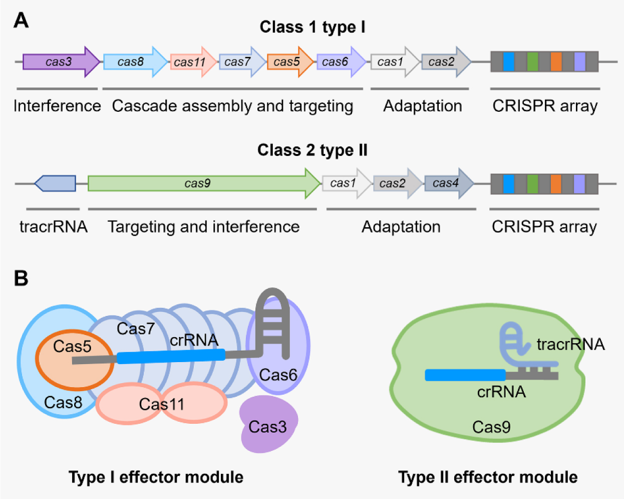
There are six major types of CRISPR-Cas systems that provide adaptive immunity in bacteria and archaea against invasive genetic elements. The discovery of CRISPR-Cas systems has revolutionized the field of genetics in many organisms. In the past few years, exploitations of the most abundant class 1 type I CRISPR-Cas systems have revealed their great potential and distinct advantages to achieve gene editing and regulation in diverse microorganisms in spite of their complicated structures. The widespread and diversified type I CRISPR-Cas systems are becoming increasingly attractive for the development of new biotechnological tools, especially in genetically recalcitrant microbial strains. In this review article, we comprehensively summarize recent advancements in microbial gene editing and regulation by utilizing type I CRISPR-Cas systems. Importantly, to expand the microbial host range of type I CRISPR-Cas-based applications, these structurally complicated systems have been improved as transferable gene-editing tools with efficient delivery methods for stable expression of CRISPR-Cas elements, as well as convenient gene-regulation tools with the prevention of DNA cleavage by obviating deletion or mutation of the Cas3 nuclease. We envision that type I CRISPR-Cas systems will largely expand the biotechnological toolbox for microbes with medical, environmental and industrial importance.
- CRISPR-Cas,
- Cascade,
- gene editing,
- gene repression,
- gene activation,
- anti-CRISPR
Citation: Zeling Xu, Shuzhen Chen, Weiyan Wu, Yongqi Wen, Huiluo Cao. Type I CRISPR-Cas-mediated microbial gene editing and regulation[J]. AIMS Microbiology, 2023, 9(4): 780-800. doi: 10.3934/microbiol.2023040

Related Papers:

Abstract

There are six major types of CRISPR-Cas systems that provide adaptive immunity in bacteria and archaea against invasive genetic elements. The discovery of CRISPR-Cas systems has revolutionized the field of genetics in many organisms. In the past few years, exploitations of the most abundant class 1 type I CRISPR-Cas systems have revealed their great potential and distinct advantages to achieve gene editing and regulation in diverse microorganisms in spite of their complicated structures. The widespread and diversified type I CRISPR-Cas systems are becoming increasingly attractive for the development of new biotechnological tools, especially in genetically recalcitrant microbial strains. In this review article, we comprehensively summarize recent advancements in microbial gene editing and regulation by utilizing type I CRISPR-Cas systems. Importantly, to expand the microbial host range of type I CRISPR-Cas-based applications, these structurally complicated systems have been improved as transferable gene-editing tools with efficient delivery methods for stable expression of CRISPR-Cas elements, as well as convenient gene-regulation tools with the prevention of DNA cleavage by obviating deletion or mutation of the Cas3 nuclease. We envision that type I CRISPR-Cas systems will largely expand the biotechnological toolbox for microbes with medical, environmental and industrial importance.

Acknowledgments

This work was supported by the National Natural Science Foundation of China (No. 32100020 and 32370188), the Guangdong Basic and Applied Basic Research Foundation (No. 2022A1515010194 and 2023A1515012775) and the Guangzhou Basic and Applied Basic Research Foundation (No. 202201010613)

Conflict of interest

The authors declare no conflict of interest.

Author contributions

Z. X. conceptualized the review topic, and S. C., W. W. and Y. W. performed the literature search. S. C. drafted the manuscript, and Z. X. and H. C. revised the manuscript. All authors read and approved the final manuscript.

References

[1]	Chandrasegaran S, Carroll D (2016) Origins of programmable nucleases for genome engineering. J Mol Biol 428: 963-989. https://doi.org/10.1016/j.jmb.2015.10.014
[2]	Fagerlund RD, Staals RHJ, Fineran PC (2015) The Cpf1 CRISPR-Cas protein expands genome-editing tools. Genome Biol 16: 251. https://doi.org/10.1186/s13059-015-0824-9
[3]	Sternberg SH, Doudna JA (2015) Expanding the biologist's toolkit with CRISPR-Cas9. Mol Cell 58: 568-574. https://doi.org/10.1016/j.molcel.2015.02.032
[4]	Barrangou R, Doudna JA (2016) Applications of CRISPR technologies in research and beyond. Nat Biotechnol 34: 933-941. https://doi.org/10.1038/nbt.3659
[5]	Zheng Y, Li J, Wang B, et al. (2020) Endogenous type I CRISPR-Cas: From foreign DNA defense to prokaryotic engineering. Front Bioeng Biotechnol 8: 62. https://doi.org/10.3389/fbioe.2020.00062
[6]	Marraffini LA, Sontheimer EJ (2008) CRISPR interference limits horizontal gene transfer in Staphylococci by targeting DNA. Science 322: 1843-1845. https://doi:10.1126/science.1165771
[7]	Barrangou R, Fremaux C, Deveau H, et al. (2007) CRISPR provides acquired resistance against viruses in prokaryotes. Science 315: 1709-1712. https://doi:10.1126/science.1138140
[8]	Nussenzweig PM, Marraffini LA (2020) Molecular mechanisms of CRISPR-Cas immunity in bacteria. Annu Rev Genet 54: 93-120. https://doi.org/10.1146/annurev-genet-022120-112523
[9]	Amitai G, Sorek R (2016) CRISPR-Cas adaptation: insights into the mechanism of action. Nat Rev Microbiol 14: 67-76. https://doi.org/10.1038/nrmicro.2015.14
[10]	Carte J, Wang R, Li H, et al. (2008) Cas6 is an endoribonuclease that generates guide RNAs for invader defense in prokaryotes. Genes Dev 22: 3489-3496. https://doi.org/10.1101/gad.1742908
[11]	Deltcheva E, Chylinski K, Sharma CM, et al. (2011) CRISPR RNA maturation by trans-encoded small RNA and host factor RNase III. Nature 471: 602-607. https://doi:10.1038/nature09886
[12]	Jore MM, Lundgren M, van Duijn E, et al. (2011) Structural basis for CRISPR RNA-guided DNA recognition by Cascade. Nat Struct Mol Bio 18: 529-536. https://doi.org/10.1038/nsmb.2019
[13]	Leenay RT, Beisel CL (2017) Deciphering, communicating, and engineering the CRISPR PAM. J Mol Biol 429: 177-191. https://doi.org/10.1016/j.jmb.2016.11.024
[14]	van der Oost J, Jore MM, Westra ER, et al. (2009) CRISPR-based adaptive and heritable immunity in prokaryotes. Trends Biochem Sci 34: 401-407. https://doi.org/10.1016/j.tibs.2009.05.002
[15]	Gasiunas G, Barrangou R, Horvath P, et al. (2012) Cas9-crRNA ribonucleoprotein complex mediates specific DNA cleavage for adaptive immunity in bacteria. Proc Natl Acad Sci U S A 109: E2579-E2586. https://doi.org/10.1073/pnas.1208507109
[16]	Westra ER, van Erp PBG, Künne T, et al. (2012) CRISPR immunity relies on the consecutive binding and degradation of negatively supercoiled invader dna by Cascade and Cas3. Mol Cell 46: 595-605. https://doi.org/10.1016/j.molcel.2012.03.018
[17]	Makarova KS, Wolf YI, Iranzo J, et al. (2020) Evolutionary classification of CRISPR-Cas systems: a burst of class 2 and derived variants. Nat Rev Microbiol 18: 67-83. https://doi.org/10.1038/s41579-019-0299-x
[18]	Makarova KS, Aravind L, Wolf YI, et al. (2011) Unification of Cas protein families and a simple scenario for the origin and evolution of CRISPR-Cas systems. Biol Direct 6: 38. https://doi.org/10.1186/1745-6150-6-38
[19]	Makarova KS, Wolf YI, Alkhnbashi OS, et al. (2015) An updated evolutionary classification of CRISPR-Cas systems. Nat Rev Microbiol 13: 722-736. https://doi.org/10.1038/nrmicro3569
[20]	Makarova KS, Wolf YI, Koonin EV (2018) Classification and nomenclature of CRISPR-Cas systems: Where from here?. CRISPR J 1: 325-336. https://doi.org/10.1089/crispr.2018.0033
[21]	Koonin EV, Makarova KS, Zhang F (2017) Diversity, classification and evolution of CRISPR-Cas systems. Curr Opin Microbiol 37: 67-78. https://doi.org/10.1016/j.mib.2017.05.008
[22]	Liu Z, Dong H, Cui Y, et al. (2020) Application of different types of CRISPR/Cas-based systems in bacteria. Microb Cell Factories 19: 172. https://doi.org/10.1186/s12934-020-01431-z
[23]	Wang Y, Huang C, Zhao W (2022) Recent advances of the biological and biomedical applications of CRISPR/Cas systems. Mol Biol Rep 49: 7087-7100. https://doi.org/10.1007/s11033-022-07519-6
[24]	Mustafa MI, Makhawi AM (2021) SHERLOCK and DETECTR: CRISPR-Cas Systems as potential rapid diagnostic tools for emerging infectious diseases. J Clin Microbiol 59: e00745-00720. https://doi.org/10.1128/jcm.00745-20
[25]	Hidalgo-Cantabrana C, Barrangou R (2020) Characterization and applications of Type I CRISPR-Cas systems. Biochem Soc Trans 48: 15-23. https://doi.org/10.1042/BST20190119
[26]	Huo Y, Nam KH, Ding F, et al. (2014) Structures of CRISPR Cas3 offer mechanistic insights into Cascade-activated DNA unwinding and degradation. Nat Struct Mol Biol 21: 771-777. https://doi.org/10.1038/nsmb.2875
[27]	Brouns SJJ, Jore MM, Lundgren M, et al. (2008) Small CRISPR RNAs guide antiviral defense in prokaryotes. Science 321: 960-964. https://doi:10.1126/science.1159689
[28]	Sinkunas T, Gasiunas G, Fremaux C, et al. (2011) Cas3 is a single-stranded DNA nuclease and ATP-dependent helicase in the CRISPR/Cas immune system. EMBO J 30: 1335-1342. https://doi.org/10.1038/emboj.2011.41
[29]	Bhatia S, Pooja, Yadav SK (2023) CRISPR-Cas for genome editing: Classification, mechanism, designing and applications. Int J Biol Macromol 238: 124054. https://doi.org/10.1016/j.ijbiomac.2023.124054
[30]	Li H (2015) Structural principles of CRISPR RNA processing. Structure 23: 13-20. https://doi.org/10.1016/j.str.2014.09.006
[31]	Wang R, Preamplume G, Terns MP, et al. (2011) Interaction of the Cas6 Riboendonuclease with CRISPR RNAs: recognition and cleavage. Structure 19: 257-264. https://doi.org/10.1016/j.str.2010.11.014
[32]	Xiao Y, Luo M, Dolan AE, et al. (2018) Structure basis for RNA-guided DNA degradation by Cascade and Cas3. Science 361: eaat0839. https://doi:10.1126/science.aat0839
[33]	Xiao Y, Luo M, Hayes RP, et al. (2017) Structure basis for directional r-loop formation and substrate handover mechanisms in type I CRISPR-Cas system. Cell 170: 48-60.e11. https://doi.org/10.1016/j.cell.2017.06.012
[34]	Semenova E, Jore MM, Datsenko KA, et al. (2011) Interference by clustered regularly interspaced short palindromic repeat (CRISPR) RNA is governed by a seed sequence. Proc Natl Acad Sci U.S.A 108: 10098-10103. https://doi.org/10.1073/pnas.1104144108
[35]	Almendros C, Nobrega FL, McKenzie RE, et al. (2019) Cas4-Cas1 fusions drive efficient PAM selection and control CRISPR adaptation. Nucleic Acids Res 47: 5223-5230. https://doi.org/10.1093/nar/gkz217
[36]	Shangguan Q, Graham S, Sundaramoorthy R, et al. (2022) Structure and mechanism of the type I-G CRISPR effector. Nucleic Acids Res 50: 11214-11228. https://doi.org/10.1093/nar/gkac925
[37]	Peters JE, Makarova KS, Shmakov S, et al. (2017) Recruitment of CRISPR-Cas systems by Tn7-like transposons. Proc Natl Acad Sci U.S.A 114: E7358-E7366. https://doi.org/10.1073/pnas.1709035114
[38]	Faure G, Shmakov SA, Yan WX, et al. (2019) CRISPR-Cas in mobile genetic elements: counter-defence and beyond. Nat Rev Microbiol 17: 513-525. https://doi.org/10.1038/s41579-019-0204-7
[39]	Hsieh SC, Peters JE (2023) Discovery and characterization of novel type I-D CRISPR-guided transposons identified among diverse Tn7-like elements in cyanobacteria. Nucleic Acids Res 51: 765-782. https://doi.org/10.1093/nar/gkac1216
[40]	Li Y, Peng N (2019) Endogenous CRISPR-Cas system-based genome editing and antimicrobials: review and prospects. Front Microbiol 10: 2471. https://doi.org/10.3389/fmicb.2019.02471
[41]	Cameron P, Coons MM, Klompe SE, et al. (2019) Harnessing type I CRISPR-Cas systems for genome engineering in human cells. Nat Biotechnol 37: 1471-1477. https://doi.org/10.1038/s41587-019-0310-0
[42]	Osakabe K, Wada N, Miyaji T, et al. (2020) Genome editing in plants using CRISPR type I-D nuclease. Commun Biol 3: 648. https://doi.org/10.1038/s42003-020-01366-6
[43]	Tan R, Krueger RK, Gramelspacher MJ, et al. (2022) Cas11 enables genome engineering in human cells with compact CRISPR-Cas3 systems. Mol Cell 82: 852-867. https://doi.org/10.1016/j.molcel.2021.12.032
[44]	Yoshimi K, Mashimo T (2022) Genome editing technology and applications with the type I CRISPR system. Gene and Genome Editing 3-4: 100013. https://doi.org/10.1016/j.ggedit.2022.100013
[45]	Osakabe K, Wada N, Murakami E, et al. (2021) Genome editing in mammalian cells using the CRISPR type I-D nuclease. Nucleic Acids Res 49: 6347-6363. https://doi.org/10.1093/nar/gkab348
[46]	Xu Z, Li Y, Li M, et al. (2021) Harnessing the type I CRISPR-Cas systems for genome editing in prokaryotes. Environ Microbiol 23: 542-558. https://doi.org/10.1111/1462-2920.15116
[47]	Hidalgo-Cantabrana C, Goh YJ, Barrangou, R (2019) Characterization and repurposing of type I and Type II CRISPR-Cas systems in bacteria. J Mol Biol 431: 21-33. https://doi.org/10.1016/j.jmb.2018.09.013
[48]	Hidalgo-Cantabrana C, Crawley AB, Sanchez B, et al. (2017) Characterization and exploitation of CRISPR Loci in Bifidobacterium longum. Front Microbiol 8: 1851. https://doi.org/10.3389/fmicb.2017.01851
[49]	Hidalgo-Cantabrana C, Goh YJ, Pan M, et al. (2019) Genome editing using the endogenous type I CRISPR-Cas system in Lactobacillus crispatus. Proc Natl Acad Sci U S A 116: 15774-15783. https://doi.org/10.1073/pnas.1905421116
[50]	Xu Z, Li Y, Yan A (2020) Repurposing the native type I-F CRISPR-Cas system in Pseudomonas aeruginosa for genome editing. STAR Protocols 1: 100039. https://doi.org/10.1016/j.xpro.2020.100039
[51]	Li Y, Pan S, Zhang Y, et al. (2016) Harnessing type I and type III CRISPR-Cas systems for genome editing. Nucleic Acids Res 44: e34. https://doi.org/10.1093/nar/gkv1044
[52]	Atmadjaja AN, Holby V, Harding AJ, et al. (2019) CRISPR-Cas, a highly effective tool for genome editing in Clostridium saccharoperbutylacetonicum N1-4(HMT). FEMS Microbiol Lett 366: fnz059. https://doi.org/10.1093/femsle/fnz059
[53]	Baker PL, Orf GS, Kevershan K, et al. (2019) Using the endogenous CRISPR-Cas system of Heliobacterium modesticaldum to delete the photochemical reaction center core subunit gene. Appl Environ Microbiol 85: e01644-01619. https://doi.org/10.1128/AEM.01644-19
[54]	Papoutsakis ET (2008) Engineering solventogenic clostridia. Curr Opin Biotechnol 19: 420-429. https://doi.org/10.1016/j.copbio.2008.08.003
[55]	McAllister KN, Sorg JA (2019) CRISPR Genome editing systems in the genus Clostridium: a timely advancement. J Bacteriol 201: e00219-00219. https://doi.org/10.1128/jb.00219-19
[56]	Pyne ME, Bruder MR, Moo-Young M, et al. (2016) Harnessing heterologous and endogenous CRISPR-Cas machineries for efficient markerless genome editing in Clostridium. Sci Rep 6: 25666. https://doi.org/10.1038/srep25666
[57]	Johnson DT, Taconi KA (2007) The glycerin glut: Options for the value-added conversion of crude glycerol resulting from biodiesel production. Environmental Progress 26: 338-348. https://doi.org/10.1002/ep.10225
[58]	Tian L, Conway PM, Cervenka ND, et al. (2019) Metabolic engineering of Clostridium thermocellum for n-butanol production from cellulose. Biotechnol Biofuels 12: 186. https://doi.org/10.1186/s13068-019-1524-6
[59]	Oka K, Osaki T, Hanawa T, et al. (2018) Establishment of an endogenous Clostridium difficile rat infection model and evaluation of the effects of Clostridium butyricum MIYAIRI 588 probiotic strain. Front Microbiol 9: 1264. https://doi.org/10.3389/fmicb.2018.01264
[60]	Hagihara M, Yamashita R, Matsumoto A, et al. (2019) The impact of probiotic Clostridium butyricum MIYAIRI 588 on murine gut metabolic alterations. J Infect Chemother 25: 571-577. https://doi.org/10.1016/j.jiac.2019.02.008
[61]	Walker JE, Lanahan AA, Zheng T, et al. (2020) Development of both type I-B and type II CRISPR/Cas genome editing systems in the cellulolytic bacterium Clostridium thermocellum. Metab Eng Commun 10: e00116. https://doi.org/10.1016/j.mec.2019.e00116
[62]	Zhou X, Wang X, Luo H, et al. (2021) Exploiting heterologous and endogenous CRISPR-Cas systems for genome editing in the probiotic Clostridium butyricum. Biotechnol Bioeng 118: 2448-2459. https://doi.org/10.1002/bit.27753
[63]	Zhang J, Zong W, Hong W, et al. (2018) Exploiting endogenous CRISPR-Cas system for multiplex genome editing in Clostridium tyrobutyricum and engineer the strain for high-level butanol production. Metab Eng 47: 49-59. https://doi.org/10.1016/j.ymben.2018.03.007
[64]	Maikova A, Kreis V, Boutserin A, et al. (2019) Using an endogenous CRISPR-Cas System for genome editing in the human pathogen Clostridium difficile. Appl Environ Microbiol 85: e01416-01419. https://doi.org/10.1128/AEM.01416-19
[65]	Dai K, Fu H, Guo X, et al. (2022) Exploiting the Type I-B CRISPR genome editing system in Thermoanaerobacterium aotearoense SCUT27 and engineering the strain for enhanced ethanol production. Appl Environ Microbiol 88: e00751-00722. https://doi.org/10.1128/aem.00751-22
[66]	Du K, Gong L, Li M, et al. (2022) Reprogramming the endogenous type I CRISPR-Cas system for simultaneous gene regulation and editing in Haloarcula hispanica. mLife 1: 40-50. https://doi.org/10.1002/mlf2.12010
[67]	Cheng F, Gong L, Zhao D, et al. (2017) Harnessing the native type I-B CRISPR-Cas for genome editing in a polyploid archaeon. J Genet Genomics 44: 541-548. https://doi.org/10.1016/j.jgg.2017.09.010
[68]	Joshi JB, Arul L, Ramalingam J, et al. (2020) Advances in the Xoo-rice pathosystem interaction and its exploitation in disease management. J Biosci 45: 112. https://doi.org/10.1007/s12038–020-00085-8
[69]	Liu Q, Wang S, Long J, et al. (2021) Functional identification of the Xanthomonas oryzae pv. oryzae Type I-C CRISPR-Cas system and its potential in gene editing application. Front Microbiol 12: 686715. https://doi.org/10.3389/fmicb.2021.686715
[70]	Jiang D, Zhang D, Li S, et al. (2022) Highly efficient genome editing in Xanthomonas oryzae pv. oryzae through repurposing the endogenous type I-C CRISPR-Cas system. Mol Plant Pathol 23: 583-594. https://doi.org/10.1111/mpp.13178
[71]	Makarova KS, Wolf YI, Koonin EV (2013) The basic building blocks and evolution of CRISPR-Cas systems. Biochem Soc Trans 41: 1392-1400. https://doi.org/10.1042/BST20130038
[72]	McBride TM, Cameron SC, Fineran PC, et al. (2023) The biology and type I/III hybrid nature of type I-D CRISPR-Cas systems. Biochem J 480: 471-488. https://doi.org/10.1042/BCJ20220073
[73]	Manav MC, Van LB, Lin J, et al. (2020) Structural basis for inhibition of an archaeal CRISPR-Cas type I-D large subunit by an anti-CRISPR protein. Nat Commun 11: 5993. https://doi.org/10.1038/s41467-020-19847-x
[74]	Bost J, Recalde A, Waßmer B, et al. (2023) Application of the endogenous CRISPR-Cas type I-D system for genetic engineering in the thermoacidophilic archaeon Sulfolobus acidocaldarius. Front Microbiol 14. https://doi.org/10.3389/fmicb.2023.1254891
[75]	Wei S, Morrison M, Yu Z (2013) Bacterial census of poultry intestinal microbiome. Poult Sci 92: 671-683. https://doi.org/10.3382/ps.2012-02822
[76]	Ravel J, Gajer P, Abdo Z, et al. (2011) Vaginal microbiome of reproductive-age women. Proc Natl Acad Sci U S A 108: 4680-4687. https://doi.org/10.1073/pnas.1002611107
[77]	Vercoe RB, Chang JT, Dy RL, et al. (2013) Cytotoxic chromosomal targeting by CRISPR/Cas systems can reshape bacterial genomes and expel or remodel pathogenicity islands. PLoS Genet 9: e1003454. https://doi.org/10.1371/journal.pgen.1003454
[78]	Hampton HG, McNeil MB, Paterson TJ, et al. (2016) CRISPR-Cas gene-editing reveals RsmA and RsmC act through FlhDC to repress the SdhE flavinylation factor and control motility and prodigiosin production in Serratia. Microbiology 162: 1047-1058. https://doi.org/10.1099/mic.0.000283
[79]	Xu Z, Li M, Li Y, et al. (2019) Native CRISPR-Cas-Mediated genome editing enables dissecting and sensitizing clinical multidrug-resistant P. aeruginosa. Cell Rep 29: 1707-1717.e1703. https://doi.org/10.1016/j.celrep.2019.10.006
[80]	Zheng Y, Han J, Wang B, et al. (2019) Characterization and repurposing of the endogenous Type I-F CRISPR-Cas system of Zymomonas mobilis for genome engineering. Nucleic Acids Res 47: 11461-11475. https://doi.org/10.1093/nar/gkz940
[81]	Hao Y, Wang Q, Li J, et al. (2022) Double nicking by RNA-directed Cascade-nCas3 for high-efficiency large-scale genome engineering. Open Biol 12: 210241. https://doi.org/10.1098/rsob.210241
[82]	Pan M, Morovic W, Hidalgo-Cantabrana C, et al. (2022) Genomic and epigenetic landscapes drive CRISPR-based genome editing in Bifidobacterium. Proc Natl Acad Sci U S A 119: e2205068119. https://doi.org/10.1073/pnas.2205068119
[83]	Marino ND, Zhang JY, Borges AL, et al. (2018) Discovery of widespread type I and type V CRISPR-Cas inhibitors. Science 362: 240-242. https://doi: 10.1126/science.aau5174
[84]	Csörgő B, León LM, Chau-Ly IJ, et al. (2020) A compact Cascade-Cas3 system for targeted genome engineering. Nat Methods 17: 1183-1190. https://doi.org/10.1038/s41592-020-00980-w
[85]	Xu Z, Li Y, Cao H, et al. (2021) A transferrable and integrative type I-F Cascade for heterologous genome editing and transcription modulation. Nucleic Acids Res 49: e94. https://doi.org/10.1093/nar/gkab521
[86]	Klompe SE, Vo PLH, Halpin-Healy TS, et al. (2019) Transposon-encoded CRISPR–Cas systems direct RNA-guided DNA integration. Nature 571: 219-225. https://doi.org/10.1038/s41586-019-1323-z
[87]	Halpin-Healy TS, Klompe SE, Sternberg SH, et al. (2020) Structural basis of DNA targeting by a transposon-encoded CRISPR-Cas system. Nature 577: 271-274. https://doi.org/10.1038/s41586-019-1849-0
[88]	Vo PLH, Ronda C, Klompe SE, et al. (2021) CRISPR RNA-guided integrases for high-efficiency, multiplexed bacterial genome engineering. Nat Biotechnol 39: 480-489. https://doi.org/10.1038/s41587-020-00745-y
[89]	Roberts A, Nethery MA, Barrangou R (2022) Functional characterization of diverse type I-F CRISPR-associated transposons. Nucleic Acids Res 50: 11670-11681. https://doi.org/10.1093/nar/gkac985
[90]	Rubin BE, Diamond S, Cress BF, et al. (2022) Species- and site-specific genome editing in complex bacterial communities. Nat Microbiol 7: 34-47. https://doi.org/10.1038/s41564-021-01014-7
[91]	Shangguan Q, White MF (2023) Repurposing the atypical type I-G CRISPR system for bacterial genome engineering. Microbiology 169. https://doi.org/10.1099/mic.0.001373
[92]	Qi LS, Larson MH, Gilbert LA, et al. (2013) Repurposing CRISPR as an rna-guided platform for sequence-specific control of gene expression. Cell 152: 1173-1183. https://doi.org/10.1016/j.cell.2013.02.022
[93]	Bikard D, Jiang W, Samai P, et al. (2013) Programmable repression and activation of bacterial gene expression using an engineered CRISPR-Cas system. Nucleic Acids Res 41: 7429-7437. https://doi.org/10.1093/nar/gkt520
[94]	Wang J, Teng Y, Zhang R, et al. (2021) Engineering a PAM-flexible SpdCas9 variant as a universal gene repressor. Nat Commun 12: 6916. https://doi.org/10.1038/s41467-021-27290-9
[95]	Luo ML, Mullis AS, Leenay RT, et al. (2015) Repurposing endogenous type I CRISPR-Cas systems for programmable gene repression. Nucleic Acids Res 43: 674-681. https://doi.org/10.1093/nar/gku971
[96]	Rath D, Amlinger L, Hoekzema M, et al. (2015) Efficient programmable gene silencing by Cascade. Nucleic Acids Res 43: 237-246. https://doi.org/10.1093/nar/gku1257
[97]	Chang Y, Su T, Qi Q, et al. (2016) Easy regulation of metabolic flux in Escherichia coli using an endogenous type I-E CRISPR-Cas system. Microb Cell Factories 15: 195. https://doi.org/10.1186/s12934-016-0594-4
[98]	Tarasava K, Liu R, Garst A, et al. (2018) Combinatorial pathway engineering using type I-E CRISPR interference. Biotechnol Bioeng 115: 1878-1883. https://doi.org/10.1002/bit.26589
[99]	Qin Z, Yang Y, Yu S, et al. (2021) Repurposing the endogenous type I-E CRISPR/Cas system for gene repression in Gluconobacter oxydans WSH-003. ACS Synth Biol 10: 84-93. https://pubs.acs.org/doi/10.1021/acssynbio.0c00456
[100]	Stachler AE, Schwarz TS, Schreiber S, et al. (2020) CRISPRi as an efficient tool for gene repression in archaea. Methods 172: 76-85. https://doi.org/10.1016/j.ymeth.2019.05.023
[101]	Maier LK, Stachler AE, Saunders SJ, et al. (2015) An active immune defense with a minimal crispr (clustered regularly interspaced short palindromic repeats) RNA and without the Cas6 protein. J Biol Chem 290: 4192-4201. https://doi.org/10.1074/jbc.M114.617506
[102]	Stachler AE, Marchfelder A (2016) Gene repression in haloarchaea using the CRISPR (clustered regularly interspaced short palindromic repeats)-Cas I-B system. J Biol Chem 291: 15226-15242. https://doi.org/10.1074/jbc.M116.724062
[103]	Chen Y, Cheng M, Song H, et al. (2022) Type I-F CRISPR-PAIR platform for multi-mode regulation to boost extracellular electron transfer in Shewanella oneidensis. iScience 25. https://doi:10.1016/j.isci.2022.104491
[104]	Marino ND, Pinilla-Redondo R, Csörgő B, et al. (2020) Anti-CRISPR protein applications: natural brakes for CRISPR-Cas technologies. Nat Methods 17: 471-479. https://doi.org/10.1038/s41592-020-0771-6
[105]	Davidson AR, Lu WT, Stanley SY, et al. (2020) Anti-CRISPRs: Protein inhibitors of CRISPR-Cas systems. Annu Rev Biochem 89: 309-332. https://doi.org/10.1146/annurev-biochem-011420-111224
[106]	Pawluk A, Shah M, Mejdani M, et al. (2017) Disabling a Type I-E CRISPR-Cas nuclease with a bacteriophage-encoded anti-crispr protein. mBio 8: 01751-01717. https://doi.org/10.1128/mbio.01751-18
[107]	Ren J, Wang H, Yang L, et al. (2022) Structural and mechanistic insights into the inhibition of type I-F CRISPR-Cas system by anti-CRISPR protein AcrIF23. J Biol Chem 298. https://doi.org/10.1016/j.jbc.2022.102124
[108]	Rollins MF, Chowdhury S, Carter J, et al. (2019) Structure reveals a mechanism of crispr-rna-guided nuclease recruitment and anti-crispr viral mimicry. Mol Cell 74: 132-142. https://doi.org/10.1016/j.molcel.2019.02.001
[109]	Chen S, Cao H, Xu Z, et al. (2023) A type I-F CRISPRi system unveils the novel role of CzcR in modulating multidrug resistance of Pseudomonas aeruginosa. Microbiol Spectr 11: e0112323. https://doi.org/10.1128/spectrum.01123-23
[110]	Li M, Gong L, Cheng F, et al. (2021) Toxin-antitoxin RNA pairs safeguard CRISPR-Cas systems. Science 372: eabe5601. https://doi:10.1126/science.abe5601
[111]	Cooper LA, Stringer AM, Wade JT (2018) Determining the specificity of cascade binding, interference, and primed adaptation in vivo in the Escherichia coli type I-E CRISPR-Cas system. mBio 9: 02100-02117. https://doi.org/10.1128/mbio.02100-18

Reader Comments

Your name:*

Email:*
© 2023 the Author(s), licensee AIMS Press. This is an open access article distributed under the terms of the Creative Commons Attribution License (http://creativecommons.org/licenses/by/4.0)