Bioactive compounds by microalgae and potentials for the management of some human disease conditions

Chijioke Nwoye Eze; Chukwu Kenechi Onyejiaka; Stella Amarachi Ihim; Thecla Okeahunwa Ayoka; Chiugo Claret Aduba; Johnson k. Ndukwe; Ogueri Nwaiwu; Helen Onyeaka; Chijioke Nwoye Eze; Chukwu Kenechi Onyejiaka; Stella Amarachi Ihim; Thecla Okeahunwa Ayoka; Chiugo Claret Aduba; Johnson k. Ndukwe; Ogueri Nwaiwu; Helen Onyeaka

doi:10.3934/microbiol.2023004

AIMS Microbiology

2023, Volume 9, Issue 1: 55-74. doi: 10.3934/microbiol.2023004

Previous Article Next Article

Review

Bioactive compounds by microalgae and potentials for the management of some human disease conditions

1.
Department of Science Laboratory Technology, University of Nigeria Nsukka
2.
Department of Microbiology, University of Nigeria Nsukka
3.
Department of Pharmacology and Toxicology, Faculty of Pharmaceutical, University of Nigeria Nsukka
4.
Department of Biochemistry, University of Nigeria Nsukka
5.
UNESCO International Centre for Biotechnology, University of Nigeria Nsukka
6.
School of Chemical Engineering, University of Birmingham, Edgbaston, Birmingham, B15 2TT, United Kingdom

Received: 09 November 2022 Revised: 18 January 2023 Accepted: 31 January 2023 Published: 07 February 2023

Microalgae biomasses are excellent sources of diverse bioactive compounds such as lipids, polysaccharides, carotenoids, vitamins, phenolics and phycobiliproteins. Large-scale production of these bioactive substances would require microalgae cultivation either in open-culture systems or closed-culture systems. Some of these bioactive compounds (such as polysaccharides, phycobiliproteins and lipids) are produced during their active growth phase. They appear to have antibacterial, antifungal, antiviral, antioxidative, anticancer, neuroprotective and chemo-preventive activities. These properties confer on microalgae the potential for use in the treatment and/or management of several neurologic and cell dysfunction-related disease conditions, including Alzheimer's disease (AD), AIDS and COVID-19, as shown in this review. Although several health benefits have been highlighted, there appears to be a consensus in the literature that the field of microalgae is still fledgling, and more research needs to be carried out to ascertain the mechanisms of action that underpin the effectiveness of microalgal compounds. In this review, two biosynthetic pathways were modeled to help elucidate the mode of action of the bioactive compounds from microalgae and their products. These are carotenoid and phycobilin proteins biosynthetic pathways. The education of the public on the importance of microalgae backed with empirical scientific evidence will go a long way to ensure that the benefits from research investigations are quickly rolled out. The potential application of these microalgae to some human disease conditions was highlighted.
- active compounds,
- carotenoids,
- Alzheimer's disease,
- oxidative stress
Citation: Chijioke Nwoye Eze, Chukwu Kenechi Onyejiaka, Stella Amarachi Ihim, Thecla Okeahunwa Ayoka, Chiugo Claret Aduba, Johnson k. Ndukwe, Ogueri Nwaiwu, Helen Onyeaka. Bioactive compounds by microalgae and potentials for the management of some human disease conditions[J]. AIMS Microbiology, 2023, 9(1): 55-74. doi: 10.3934/microbiol.2023004

Related Papers:

Abstract

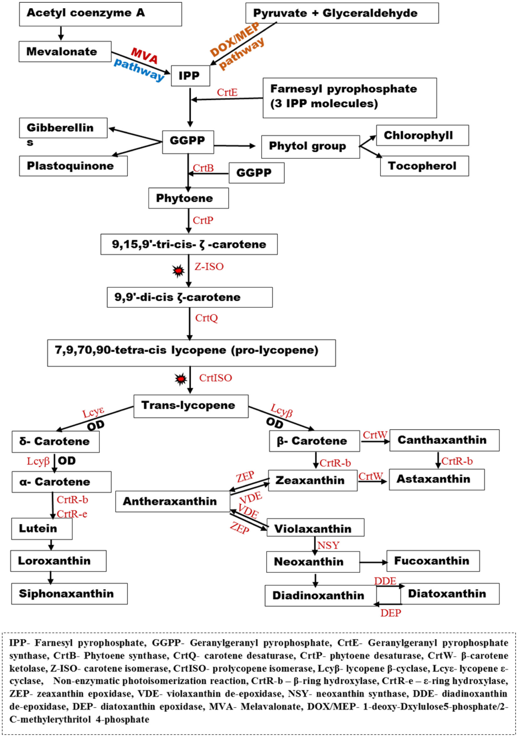
Microalgae biomasses are excellent sources of diverse bioactive compounds such as lipids, polysaccharides, carotenoids, vitamins, phenolics and phycobiliproteins. Large-scale production of these bioactive substances would require microalgae cultivation either in open-culture systems or closed-culture systems. Some of these bioactive compounds (such as polysaccharides, phycobiliproteins and lipids) are produced during their active growth phase. They appear to have antibacterial, antifungal, antiviral, antioxidative, anticancer, neuroprotective and chemo-preventive activities. These properties confer on microalgae the potential for use in the treatment and/or management of several neurologic and cell dysfunction-related disease conditions, including Alzheimer's disease (AD), AIDS and COVID-19, as shown in this review. Although several health benefits have been highlighted, there appears to be a consensus in the literature that the field of microalgae is still fledgling, and more research needs to be carried out to ascertain the mechanisms of action that underpin the effectiveness of microalgal compounds. In this review, two biosynthetic pathways were modeled to help elucidate the mode of action of the bioactive compounds from microalgae and their products. These are carotenoid and phycobilin proteins biosynthetic pathways. The education of the public on the importance of microalgae backed with empirical scientific evidence will go a long way to ensure that the benefits from research investigations are quickly rolled out. The potential application of these microalgae to some human disease conditions was highlighted.

Conflict of interest

The authors declare no conflict of interest.

Author contributions

CNE: writing; CKO: writing; SAI: writing; TOA: writing; CCA: writing and editing; JKN: writing and editing; ON: supervision and editing; HO: review and analysis of the final draft.

References

[1]	Sathasivam R, Ki JS (2018) A review of the biological activities of microalgal carotenoids and their potential use in healthcare and cosmetic industries. Mar Drugs 16: 1-31. https://doi.org/10.3390/md16010026
[2]	Koyande AK, Chew KW, Rambabo K, et al. (2019) Microalgae: a potential alternative to health supplementationfor humans. Food Sci Human Wellness 8: 16-24. https://doi.org/10.1016/j.fshw.2019.03.001
[3]	Mangialasche F, Westman E, Kivipelto M, et al. (2013) Classification and prediction of clinical diagnosis of Alzheimer's disease based on MRI and plasma measures of α-/γ-tocotrienols and γ-tocopherol. J Intern Med 273: 602-621. https://doi.org/10.1111/joim.12037
[4]	Sasaki K, Geribaldi-Doldán N, Wu Q, et al. (2021) Microalgae Aurantiochytrium Sp. increases neurogenesis and improves spatial learning and memory in senescence-accelerated mouse-prone 8 mice. Front Cell Dev Biol 8: 600575. https://doi.org/10.3389/fcell.2020.600575
[5]	Sathasivam R, Radhakrishnan R, Hashem A, et al. (2019) Microalgae metabolites: a rich source for food and medicine. Saudi J Biol Sci 26: 709-722. https://doi.org/10.1016/j.sjbs.2017.11.003
[6]	Eze CN, Aoyagi H, Ogbonna JC (2020) Simultaneous accumulation of lipid and carotenoid in freshwater green microalgae Desmodesmus subspicatus LC172266 by nutrient replete strategy under mixotrophic condition. Korean J Chem Eng 37: 1522-1529. https://doi.org/10.1007/s11814-020-0564-8
[7]	Pham-Huy LA, He H, Pham-Huy C (2008) Free radicals, antioxidants in disease and health. Int J Biomed Sci 4: 89-96.
[8]	Dehghani J, Movafeghi A, Mathieu-Rivet E, et al. (2022) Microalgae as an efficient vehicle for the production and targeted delivery of therapeutic glycoproteins against SARS-CoV-2 variants. Mar Drugs 20: 657. https://doi.org/10.3390/md20110657
[9]	Ataie A, Shadifar M, Ataee R (2016) Polyphenolic antioxidants and neuronal regeneration. Basic Clinic Neurosci 7: 81-90. https://doi.org/10.15412/J.BCN.03070201
[10]	Bule MH, Ahmed I, Maqboil F, et al. (2018) Microalgae as a source of high-value bioactive compounds. Front Biosci 10: 197-216. https://doi.org/10.2741/s509
[11]	Santosh S, Dhandapani R, Hemalatha N (2016) Bioactive compounds from microalgae and its different application–a review. Adv Appl Sci Res 7: 153-158.
[12]	Olasehinde TA, Olaniran AO, Anthony I, et al. (2017) Therapeutic potentials of microalgae in the treatment of Alzheimer's disease. Molecules 22: 1-18. https://doi.org/10.3390/molecules22030480
[13]	Tamiya H (1957) Mass cultivation of algae. Ann Rev Plant Physiol 8: 309-344.
[14]	Eze CN, Ogbonna IO, Aoyagi H, et al. (2021) Comparison of growth, protein and carotenoid contents of some freshwater microalgae and effects of urea and cultivation in a photobioreactor with reflective broth circulation guide on Desmodesmus subspicatus LC172266. Braz J Chem Engin 39: 23-33. https://doi.org/10.1007/s43153-021-00120-7
[15]	Egbo MK, Okoani AO, Okoh IE (2018) Photobioreactors for microalgae cultivation – an overview. Int J Scient Engin Res 9: 65-74.
[16]	Borowitzka MA (1996) Closed algal photobioreactors: design considerations for large scale systems. J Mar Biotechnol 4: 185-191.
[17]	Eze CN, Ogbonna JC, Ogbonna IO, et al. (2017) A novel flat plate air-lift photobioreactor with inclined reflective broth circulation guide for improved biomass and lipid productivity by Desmodesmus subspicatus LC172266. J Appl Phycol 29: 2745-2754. https://doi.org/10.1007/s10811-017-1153-z
[18]	Aratboni HA, Rafiel N, Garcia-Granados R, et al. (2019) Biomass and lipid induction strategies in microalgae for biofuel production and other applications. Microb Cell Fact 18: 178. https://doi.org/10.1186/s12934-019-1228-4
[19]	Ma R, Zhao X, Xie Y, et al. (2019) Enhancing lutein productivity of Chlamydomonas sp. via high-intensity light exposure with corresponding carotenogenic genes expression profiles. Bioresour Technol 275: 416-420. https://doi.org/10.1016/j.biortech.2018.12.109
[20]	Patel AK, Joun JM, Hong ME, et al. (2019) Effect of light conditions on mixotrophic cultivation of green microalgae. Bioresour Technol 282: 245-253. https://doi.org/10.1016/j.biortech.2019.03.024
[21]	Dario PP, Balmant W, Lírio FR, et al. (2021) Lumped intracellular dynamics: Mathematical modeling of the microalgae Tetradesmus obliquus cultivation under mixotrophic conditions with glycerol. Algal Res 57: 102344. https://doi.org/10.1016/j.algal.2021.102344
[22]	Guo W, Zhu S, Li S, et al. (2021) Microalgae polysaccharides ameliorates obesity in association with modulation of lipid metabolism and gut microbiota in high-fat-diet fed C57BL/6 mice. Int J Biol Macromol 182: 1371-1383. https://doi.org/10.1016/j.ijbiomac.2021.05.067
[23]	Tripathi S, Kairamkonda M, Gupta P, et al. (2023) Dissecting the molecular mechanisms of producing biofuel and value-added products by cadmium tolerant microalgae as sustainable biorefinery approach. Chem Eng J 454: 140068. https://doi.org/10.1016/j.cej.2022.140068
[24]	Agbebi TV, Ojo EO, Watson IA (2022) Towards optimal inorganic carbon delivery to microalgae culture. Algal Res 67: 102841. https://doi.org/10.1016/j.algal.2022.102841
[25]	Chen JH, Chen CY, Hasunuma T, et al. (2019) Enhancing lutein production with mixotrophic cultivation of Chlorella sorokiniana MB-1-M12 using different bioprocess operation strategies. Bioresour Technol 278: 17-25. https://doi.org/10.1016/j.biortech
[26]	Hanschen ER, Shawn RS (2020) The state of algal genome quality and diversity. Algal Res 50: 101968. https://doi.org/10.1016/j.algal.2020.101968
[27]	Miralles A, Teddy B, Katherine W, et al. (2020) Repository for taxonomic data: where we are and what we are missing. Syst Biol 69: 1231-1253. https://doi.org/10.1093/sysbio/syaa026
[28]	Bringloe TT, Samuel S, Rachael MW, et al. (2020) Phylogeny and Evolution of the Brown Algae. Crit Rev Plant Sci 39: 281-321. https://doi.org/10.1080/07352689.2020.1787679
[29]	de Sousa BC, Cox CJ, Brito L, et al. (2019) Improved phylogeny of brown algae Cystoseira (Fucales) from the Atlantic-Mediterranean region based on mitochondrial sequences. PLoS ONE 14: e0210143. https://doi.org/10.1371/journal.pone.0210143
[30]	Savoie AM, Ssaunders GW (2018) A molecular assessment of species diversity and generic boundaries in the red algal tribes Polysiphonieae and Streblocladieae (Rhodomelaceae, Rhodophyta) in Canada. Eur J Phycol 54: 1-25. https://doi.org/10.1080/09670262.2018.1483531
[31]	Saghel A, Kongkana G, Pal M, et al. (2019) Morpho-taxonomic, genetic, and biochemical characterization of freshwater microalgae as potential biodiesel feedstock. 3 Biotech 9: 137. https://doi.org/10.1007/s13205-019-1664-1
[32]	Gonulol A, Ersanli E, Baytut O (2009) Taxonomical and numerical comparison of epipelic algae from Balik and Uzun lagoon, Turkey. J Environ Biol 30: 777-784.
[33]	Welker M, Dittmann E, von Dohren H (2012) Cyanobacteria as a source of natural products. Method Enzymol 517: 23-46. https://doi.org/10.1016/B978-0-12-404634-4.00002-4
[34]	Munir N, Sharif N, Naz S, et al. (2013) Algae: a potent antioxidant source. Sky J Microbiol Res 1: 22-31.
[35]	Fu W, Nelson DR, Yi Z, et al. (2017) Bioactive compounds from microalgae: current development and prospects. Studies in Natural Products Chemistry.Elsevier 199-225. https://doi.org/10.1016/B978-0-444-63929-5.00006-1
[36]	Elufioye TO, Chinaka CG, Oyedeji AO (2019) Antioxidant and anticholinesterase activities of Macrosphyra Longistyla (DC) hiern relevant in the management of Alzheimer's disease. Antioxidant 8: 1-15. https://doi.org/10.3390/antiox8090400
[37]	Alam MA, Parra-Saldivar R, Bilal M, et al. (2021) Algae-derived bioactive molecules for the potential treatment of SARS-CoV-2. Molecules 26: 1-16. https://doi.org/10.3390/molecules26082134
[38]	Gulçin I, Oktay M, Kufrevioglu OI, et al. (2002) Determination of antioxidant activity of lichen Cetraria islandica (L) Ach. J Ethno-pharmacol 79: 325-329. https://doi.org/10.1016/S0378-8741(01)00396-8
[39]	Halliwell B (2006) Reactive species and antioxidants. redox biology is a fundamental theme of aerobic life. Plant Physiol 41: 312-322. https://doi.org/10.1104/pp.106.077073
[40]	Gill SS, Tuteja N (2010) Reactive oxygen species and antioxidant machinery in abiotic stress tolerance in crop plants. Plant Physiol Biochem 48: 909-930. https://doi.org/10.1016/j.plaphy.2010.08.016
[41]	Tewari RK, Kumar P, Sharma PN (2006) Antioxidant responses to enhanced generation of superoxide anion radical and hydrogen peroxide in the copper-stressed mulberry plants. Planta 223: 1145-1153. https://doi.org/10.1007/s00425-005-0160-5
[42]	Wright SW, Jeffrey SW (2006) Pigment markers for phytoplankton production. Marine Organic Matter: Biomarkers, Isotopes and DNA. Berlin: Springer 71-104.
[43]	Fasnacht M, Polacek N (2021) Oxidative stress in bacteria and the central dogma of molecular biology. Front Molec Biosci 8: 1-13. https://doi.org/10.3389/fmolb.2021.671037
[44]	Filiz E, Ozyigit II, Saracoglu IA, et al. (2019) Abiotic stress-induced regulation of antioxidant genes in different Arabidopsis ecotypes: microarray data evaluation. Biotechnol Biotechnologic Equip 33: 1-16. https://doi.org/10.1080/13102818.2018.1556120
[45]	Manning SR, Nobles DR (2017) Impact of global warming on water toxicity: cyanotoxins. Curr Opinions Food Sci 18: 14-20. https://doi.org/10.1016/j.cofs.2017.09.013
[46]	Bhosale P (2004) Environmental and cultural stimulants in the production of carotenoids from microorganisms. Appl Microb Biotechnol 63: 351-361. https://doi.org/10.1007/s00253-003-1441-1
[47]	Takaichi S (2011) Carotenoids in algae: distributions, biosyntheses and functions. Marine Drugs 9: 1101-1118. https://doi.org/10.3390/md9061101
[48]	Wilson GM, Gorgich M, Corrêa PS, et al. (2020) Microalgae for biotechnological applications. Cultivation, harvesting and biomass processing. Aquaculture 528: 735562. https://doi.org/10.1016/j.aquaculture.2020.735562
[49]	Vuppaladadiyam AK, Prinsen P, Raheem A, et al. (2018) Microalgae cultivation and metabolites production: a comprehensive review. Biofuel Bioprod Bioref 12: 304-324. https://doi.org/10.1002/bbb.1864
[50]	Tamaki S, Mochida K, Suzuki K (2021) Diverse biosynthetic pathways and protective functions against environmental stress of antioxidants in microalgae. Plants 10: 1-17. https://doi.org/10.3390/plants10061250
[51]	Huang JJ, Lin S, Xu W, et al. (2017) Occurrence and biosynthesis of carotenoids in phytoplankton. Biotechnol Adv 35: 597-618. https://doi.org/10.1016/j.biotechadv.2017.05.001
[52]	Takaichi S (2020) Carotenoids in phototrophic microalgae: distributions and biosynthesis. Pigments from Microalgae Handbook. Switzerland: Springer: Cham 19-42. https://doi.org/10.1007/978-3-030-50971-2_2
[53]	Grossman AR, Lohr M, Im CS (2004) Chlamydomonas reinhardtii in the landscape of pigments. Ann Rev Genetics 38: 119-173. https://doi.org/10.1146/annurev.genet.38.072902.092328
[54]	Rodríguez-Villalón A, Gas E, Rodríguez-Concepción M (2009) Phytoene synthase activity controls the biosynthesis of carotenoids and the supply of their metabolic precursors in dark-grown Arabidopsis seedlings. Plant Journal 60: 424-435. https://doi.org/10.1111/j.1365-313X.2009.03966.x
[55]	Li W, Su H, Pu Y, et al. (2019) Phycobiliproteins: molecular structure, production, applications, and prospects. Biotechnol Adv 37: 340-353. https://doi.org/10.1016/j.biotechadv.2019.01.008
[56]	Zaffagnini M, Bedhomme M, Groni H, et al. (2012) Glutathionylation in the photosynthetic model organism Chlamydomonas reinhardtii: A proteomic survey. Molecul Cellul Proteom 11: 1-15. https://doi.org/10.1074/mcp.M111.014142–2
[57]	Alemanno A, Garde A (2013) The emergence of an EU lifestyle policy: the case of alcohol, tobacco and unhealthy diets. Common Market Law Rev 6: 1745-1786. https://doi.org/10.54648/COLA2013165
[58]	Ejike CE, Collins SA, Balasuriya N, et al. (2017) Prospects of microalgae proteins in producing peptide-based functional foods for promoting cardiovascular health. Trends Food Sci Technol 59: 30-36. https://doi.org/10.1016/j.tifs.2016.10.026
[59]	Galasso C, Gentile A, Orefice I, et al. (2019) Microalgal derivatives as potential nutraceutical and food supplements for human health: A focus on cancer prevention and interception. Nutrients 11: 1-22. https://doi.org/10.3390/nu11061226
[60]	Hoseinifar SH, Yousefi S, Capillo G, et al. (2018) Mucosal immune parameters, immune and antioxidant defence related genes expression and growth performance of zebrafish (Danio rerio) fed on Gracilaria gracilis powder. Fish Shellfish Immunol 83: 232-237. https://doi.org/10.1016/j.fsi.2018.09.046
[61]	Capillo G, Savoca S, Costa R, et al. (2018) New insights into the culture method and antibacterial potential of Gracilaria gracilis. Marine Drugs 16: 492. https://doi.org/10.3390/md16120492
[62]	Pereira L, Critchley AT (2020) The COVID 19 novel coronavirus pandemic 2020: Seaweeds to the rescue? Why does substantial, supporting research about the antiviral properties of seaweed polysaccharides seem to go unrecognized by the pharmaceutical community in these desperate times?. J Appl Phycol 32: 1875-1877. https://doi.org/10.1007/s10811-020-02143-y
[63]	Wang W, Wang SX, Guan HS (2012) The antiviral activities and mechanisms of marine polysaccharides: an overview. Marine Drugs 10: 2795-2816. https://doi.org/10.3390/md10122795
[64]	Chen X, Han W, Wang G, et al. (2020) Application prospect of polysaccharides in the development of anti-novel coronavirus drugs and vaccines. Int J Biol Macromolec 164: 331-343. https://doi.org/10.1016/j.ijbiomac.2020.07.106
[65]	Sanniyasi E, Venkatasubramanian G, Anbalagan MM, et al. (2019) In vitro anti-HIV-1 activity of the bioactive compound extracted and purified from two different marine macroalgae (seaweeds) (Dictyota bartayesiana JV Lamouroux and Turbinaria decurrens Bory). Sci Rep 9: 1-12. https://doi.org/10.1038/s41598-019-47917-8
[66]	Joseph J, Thankamani K, Ajay A, et al. (2020) Green tea and Spirulina extracts inhibit SARS, MERS, and SARS-2 spike pseudo-typed virus entry in vitro. bioRxiv 1–28. https://doi.org/10.1101/2020.06.20.162701
[67]	Ko SC, Kim D, Jeon YJ (2012) Protective effect of a novel antioxidative peptide purified from a marine Chlorella ellipsoidea protein against free radical-induced oxidative stress. Food Chem Toxicol 50: 2294-2302. https://doi.org/10.1016/j.fct.2012.04.022
[68]	Sheih IC, Wu TK, Fang TJ (2009) Antioxidant properties of a new antioxidative peptide from algae protein waste hydrolysate in different oxidation systems. Bioresour Technol 100: 3419-3425. https://doi.org/10.1016/j.biortech.2009.02.014
[69]	Cerón MC, García-Malea MC, Rivas J, et al. (2007) Antioxidant activity of Haematococcus pluvialis cells grown in continuous culture as a function of their carotenoid and fatty acid content. Appl Microbiol Biotechnol 74: 1112-1119. https://doi.org/10.1007/s00253-006-0743-5
[70]	Goiris K, Muylaert K, Fraeye I, et al. (2012) Antioxidant potential of microalgae in relation to their phenolic and carotenoid content. J Appl Phycol 24: 1477. https://doi.org/10.1007/s10811-012-9804-6
[71]	Barros MP, Poppe SC, Bondan EF (2014) Neuroprotective properties of the marine carotenoid astaxanthin and omega-3 fatty acids, and perspectives for the natural combination of both in krill oil. Nutrients 6: 1293-1317. https://doi.org/10.3390/nu6031293
[72]	Dyall SC (2015) Long-chain omega-3 fatty acids and the brain: A review of the independent and shared effects of EPA, DPA and DHA. Front Aging Neurosci 7: 1-15. https://doi.org/10.3389/fnagi.2015.00052
[73]	Talero E, García-Mauriño S, Ávila-Román J, et al. (2015) Bioactive compounds isolated from microalgae in chronic inflammation and cancer. Marine Drugs 13: 6152-6209. https://doi.org/10.3390/md13106152
[74]	Luo X, Su P, Zhang W (2015) Advances in microalgae-derived phytosterols for functional food and pharmaceutical applications. Marine Drugs 13: 4231-4254. https://doi.org/10.3390/md13074231
[75]	Custódio L, Justo T, Silvestre L, et al. (2012) Microalgae of different phyla display antioxidant, metal chelating and acetylcholinesterase inhibitory activities. Food Chem 131: 134-140. https://doi.org/10.1016/j.foodchem.2011.08.047
[76]	Oboh G, Nwanna EE, Oyeleye SI, et al. (2016) In vitro neuroprotective potentials of aqueous and methanol extracts from Heinsia crinita leaves. Food Sci Human Wellness 5: 95-102. https://doi.org/10.1016/j.fshw.2016.03.001
[77]	Aluko RE (2021) Food-derived acetylcholinesterase inhibitors as potential agents against Alzheimer's disease. Food 2: 49-58. https://doi.org/10.2991/efood.k.210318.001
[78]	Olasehinde TO, Olaniran AO, Okoh AI (2020) Cholinesterase inhibitory activity, antioxidant properties, and phytochemical composition of Chlorococcum sp. extracts. J Food Chem 45: e13395. https://doi.org/10.1111/jfbc.13395
[79]	Cortes N, Posada-Duque RA, Alvarez R, et al. (2015) Neuroprotective activity and acetylcholinesterase inhibition of five Amaryllidaceae species: a comparative study. Life Sci 122: 42-50. https://doi.org/10.1016/j.lfs.2014.12.011
[80]	Chon S, Yang E, Lee T, et al. (2016) β-Secretase (BACE1) inhibitory and neuroprotective effects of p-terphenyls from Polyozellus multiplex. Food Funct 7: 3834-3842. https://doi.org/10.1039/c6fo00538a
[81]	Zhou L, Li K, Duan X, et al. (2022) Bioactive compounds in microalgae and their potential health benefits. Food Biosci 49: 101932. https://doi.org/10.1016/j.fbio.2022.101932
[82]	Garofalo C, Norici A, Mollo L, et al. (2022) Fermentation of microalgal biomass for innovative food production. Microorg 10: 2069. https://doi.org/10.3390/microorganisms10102069
[83]	Silva M, Kamberovic F, Uota ST, et al. (2022) Microalgae as potential sources of bioactive compounds for functional foods and pharmaceuticals. Appl Sci 12: 5877. https://doi.org/10.3390/app12125877
[84]	El Nemr A, Shobier AH, El Ashry S, et al. (2021) Pharmacological screening of some Egyptian marine algae and encapsulation of their bioactive extracts in calcium alginate beads. Egy J Aquatic Biol Fisheries 25: 1025-1052. https://doi.org/10.21608/EJABF.2021.170631
[85]	Hassaan MA, El Nemr A, Elkatory MR, et al. (2021) Enhancement of biogas production from macroalgae U. Lactuca via ozonation pre-treatment. Energ 14: 1703. https://doi.org/10.3390/en14061703
[86]	Andrade LM, Andrade CJ, Dias M, et al. (2018) Chlorella and spirulina microalgae as sources of functional foods, nutraceuticals, and food supplements: an overview. MOJ Food Proc Technol 6: 45-58. https://doi.org/10.15406/MOJFPT.2018.06.00144
[87]	Barkia I, Saari N, Manning SR (2019) Microalgae for high-value products towards human health and nutrition. Marine Drugs 17: 1-29. https://doi.org/10.3390/md17050304
[88]	Gong M, Bassi A (2016) Carotenoids from microalgae: a review of recent developments. Biotechnol Adv 34: 1396-1412. https://doi.org/10.1016/j.biotechadv.2016.10.005
[89]	Sánchez JF, Fernández-Sevilla JM, Acién FG, et al. (2008) Biomass and lutein productivity of Scenedesmus almeriensis: Influence of irradiance, dilution rate and temperature. Appl Microbiol Biotechnol 79: 719-729. https://doi.org/10.1007/s00253-008-1494-2
[90]	Cordero BF, Obraztsova I, Couso I, et al. (2011) Enhancement of lutein production in Chlorella sorokiniana (Chorophyta) by improvement of culture conditions and random mutagenesis. Marine Drugs 9: 1607-1624. https://doi.org/10.3390/md9091607
[91]	Guerin M, Huntley ME, Olaizola M (2003) Haematococcus astaxanthin: applications for human health and nutrition. Trends Biotechnol 21: 210-216. https://doi.org/10.1016/S0167-7799(03)00078-7
[92]	Cai X, Chen Y, Xie X, et al. (2019) Astaxanthin prevents against lipopolysaccharide-induced acute lung injury and sepsis via inhibiting activation of MAPK/NF-kB. Amer J Translation Res 11: 1884-1894.
[93]	Capelli R, Talbott S, Ding L (2019) Astaxanthin sources: suitability for human health and nutrition. Function Foods Health Dis 9: 430-445. https://doi.org/10.31989/ffhd.v9i6.584
[94]	Park JS, Chyun JH, Kim YK, et al. (2010) Astaxanthin decreased oxidative stress and inflammation and enhanced immune response in humans. Nutrition Metabol 7: 18. https://doi.org/10.1186/1743-7075-7-18
[95]	Wu Q, Zhang XS, Wang HD, et al. (2014) Astaxanthin activates nuclear factor erythroid-related factor 2 and the antioxidant responsive element (Nrf2-ARE) pathway in the brain after subarachnoid hemorrhage in rats and attenuates early brain injury. Marine Drugs 12: 6125-6141. https://doi.org/10.3390/md12126125
[96]	Koller M, Muhr A, Braunegg G (2014) Microalgae as versatile cellular factories for valued products. Algal Res 6: 52-63. https://doi.org/10.1016/j.algal.2014.09.002
[97]	Bishop WM, Zubeck HM (2012) Evaluation of microalgae for use as nutraceuticals and nutritional supplements. J Nutrition Food Sci 2: 147. https://doi.org/10.4172/2155-9600.1000147
[98]	Sonani RR, Rastogi RP, Patel R, et al. (2016) Recent advances in production, purification and applications of phycobiliproteins. World J Biol Chem 7: 100-109. https://doi.org/10.4331/wjbc.v7.i1.100
[99]	Magdugo RP, Terme N, Lang M, et al. (2020) An analysis of the nutritional and health values of Caulerpa racemosa (Forsskål) and Ulva fasciata (Delile)—two chlorophyta collected from the Philippines. Molecules 25: 1-23. https://doi.org/10.3390/molecules25122901
[100]	Chénais B (2021) Algae and microalgae and their bioactive molecules for human health. Molecules 26: 1-4. https://doi.org/10.3390/molecules26041185
[101]	Orejuela-Escobar L, Gualle A, Ochoa-Herrera V, et al. (2021) Prospects of microalgae for biomaterial production and environmental applications at biorefineries. Sustainability 13: 1-19. https://doi.org/10.3390/su13063063
[102]	Kim SK, Kang KH (2011) Medicinal effects of peptides from marine microalgae. Adv Food Nutrition Resour 64: 313-323. https://doi.org/10.1016/B978-0-12-387669-0.00025-9
[103]	Lawrence KP, Long PF, Young AR (2018) Mycosporine-like amino acids for skin photoprotection. Curr Med Chem 25: 5512-5527. https://doi.org/10.2174/0929867324666170529124237
[104]	Odjadjare EC, Mutanda T, Olaniran AO (2017) Potential biotechnological application of microalgae: a critical review. Crit Rev Biotechnol 37: 37-52. https://doi.org/10.3109/07388551.2015.1108956
[105]	Khanra S, Mondal M, Halderl G, et al. (2018) Downstream processing of microalgae for pigments, protein and carbohydrate in industrial application: a review. Food Bioprod Process 110: 60-84. https://doi.org/10.1016/j.fbp.2018.02.002
[106]	Becker EW (2004) Microalgae in human and animal nutrition. Handbook of micro algal culture. Oxford: Blackwell 312-351.
[107]	Carballo-Cardenas EC, Tuan PM, Janssen M, et al. (2003) Vitamin E (alpha-tocopherol) production by the marine microalgae Dunaliella tertiolecta and Tetraselmis suecica in batch cultivation. Biomolecul Engin 20: 139-147. https://doi.org/10.1016/S1389-0344(03)00040-6
[108]	Matsukawa R, Hotta M, Masuda Y, et al. (2000) Antioxidants from carbon dioxide fixing Chlorella sorokiniana. J Appl Phycol 12: 263-267. https://doi.org/10.1023/A:1008141414115
[109]	Giammanco M, Di Majo D, La Guardia M, et al. (2015) Vitamin D in cancer chemoprevention. Pharmaceutical Biol 53: 1399-1434. https://doi.org/10.3109/13880209.2014.988274
[110]	Bong SC, Loh SP (2013) A study of fatty acid composition and tocopherol content of lipid extracted from marine microalgae, Nannochloropsis oculata and Tetraselmis suecica, using solvent extraction and supercritical fluid extraction. Int Food Res J 20: 721-729.
[111]	Santiago-Morales IS, Trujillo-Valle L, Márquez-Rocha FJ, et al. (2018) Tocopherols, phycocyanin and superoxide dismutase from microalgae as potential food anti-oxidants. Appl Food Biotechnol 5: 19-27. https://doi.org/10.22037/afb.v5i1.17884
[112]	Khalid S, Abbas M, Saeed F, et al. (2018) Therapeutic potential of seaweed bioactive compounds. Seaweed Biomater 1: 7-26. https://doi.org/10.5772/INTECHOPEN.74060
[113]	Kelman D, Posner EK, McDermid KJ, et al. (2012) Antioxidant activity of Hawaiian marine algae. Marine Drugs 10: 403-416. https://doi.org/10.3390/md10020403
[114]	Guedes AC, Amaro HM, Malcata FX (2011) Microalgae as sources of high added-value compounds—a brief review of recent work. Biotechnol Prog 27: 597-613. https://doi.org/10.1002/btpr.575
[115]	Lohrmann NL, Logan BA, Johnson AS (2004) Seasonal acclimatization of antioxidants and photosynthesis in Chondrus crispus and Mastocarpus stellatus, two co-occurring red algae with differing stress tolerances. Biol Bulletin 207: 225-232. https://doi.org/10.2307/1543211
[116]	Ebrahimzadeh MA, Khalili M, Dehpour AA (2018) Antioxidant activity of ethyl acetate and methanolic extracts of two marine algae, Nannochloropsis oculata and Gracilaria gracilis-an in vitro assay. Braz J Pharmaceut Sci 54: 17280. https://doi.org/10.1590/s2175-97902018000117280
[117]	Cornish ML, Garbary DJ (2010) Antioxidants from macroalgae: Potential applications in human health and nutrition. Algae 25: 155-171. https://doi.org/10.4490/algae.2010.25.4.155
[118]	Delattre C, Pierre G, Laroche C, et al. (2016) Production, extraction and characterization of microalgal and cyanobacterial exopolysaccharides. Biotechnol Adv 34: 1159-1179. https://doi.org/10.1016/j.biotechadv.2016.08.001
[119]	Xiao R, Zheng Y (2016) Overview of microalgal extracellular polymeric substances (EPS) and their applications. Biotechnol Adv 34: 1225-1244. https://doi.org/10.1016/j.biotechadv.2016.08.004
[120]	Farah A, De Paulis T, Trugo LC, et al. (2005) Effect of roasting on the formation of chlorogenic acid lactones in coffee. J Agri Food Chem 53: 1505-1513. https://doi.org/10.1021/jf048701t
[121]	Kweon MH, Hwang HJ, Sung HC (2001) Identification and antioxidant activity of novel chlorogenic acid derivatives from bamboo (Phyllostachys edulis). J Agric Food Chem 49: 4646-4655. https://doi.org/10.1021/jf010514x
[122]	Robinson WE, Reinecke MG, Abdel-Malek S, et al. (1996) Inhibitors of HIV-1 replication that inhibit HPV integrase. Proc Nation Acad Sci USA 93: 6326-6331. https://doi.org/10.1073/PNAS.93.13.6326
[123]	Kwon HC, Jung CM, Shin CG, et al. (2000) A new caffeoyl quinic acid from Aster scaber and its inhibitory activity against human immunodeficiency virus-1 (HIV-1) integrase. Chem Pharmaceut Bulletin 48: 1796-1798. https://doi.org/10.1248/CPB.48.1796
[124]	Asgharpour M, Rodgers B, Hestekin JA (2015) Eicosapentaenoic acid from Porphyridium Cruentum: Increasing growth and productivity of microalgae for pharmaceutical products. Energies 8: 10487-10503. https://doi.org/10.3390/en80910487

Reader Comments

Your name:*

Email:*
© 2023 the Author(s), licensee AIMS Press. This is an open access article distributed under the terms of the Creative Commons Attribution License (http://creativecommons.org/licenses/by/4.0)