Currently, most network outages occur because of manual configuration errors. Therefore, it is essential to verify the correctness of network configurations before deployment. Computing the network control plane is a key technology for network configuration verification. We can verify the correctness of network configurations for fault tolerance by generating routing tables, as well as connectivity. However, existing routing table calculation tools have disadvantages such as lack of user-friendliness, limited expressiveness, and slower speed of routing table generation. In this paper, we present FastCAT, a framework for computing routing tables incorporating multiple protocols. FastCAT can simulate the interaction of multiple routing protocols and quickly generate routing tables based on configuration files and topology information. The key to FastCAT's performance is that FastCAT focuses only on the final stable state of the OSPF and IS-IS protocols, disregarding the transient states during protocol convergence. For RIPv2 and BGP, FastCAT computes the current protocol routing tables based on the protocol's previous state, retaining only the most recent protocol routing tables in the latest state. Experimental evaluations have shown that FastCAT generates routing tables more quickly and accurately than the state-of-the-art routing simulation tool, in a general network of around 200 routers.
Citation: Jianfei Cai, Guozheng Yang, Jingju Liu, Yi Xie. FastCAT: A framework for fast routing table calculation incorporating multiple protocols[J]. Mathematical Biosciences and Engineering, 2023, 20(9): 16528-16550. doi: 10.3934/mbe.2023737
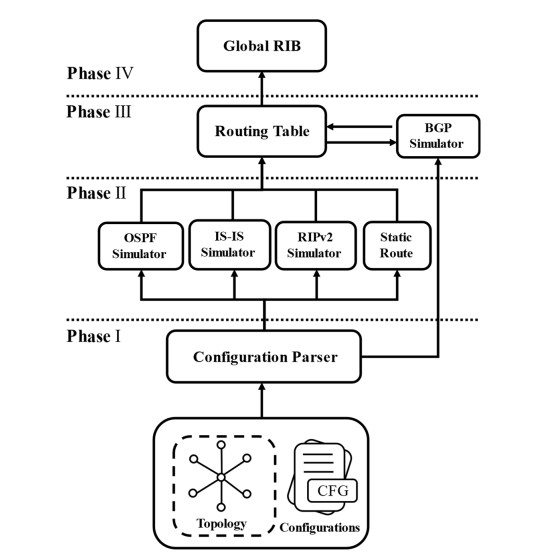
Currently, most network outages occur because of manual configuration errors. Therefore, it is essential to verify the correctness of network configurations before deployment. Computing the network control plane is a key technology for network configuration verification. We can verify the correctness of network configurations for fault tolerance by generating routing tables, as well as connectivity. However, existing routing table calculation tools have disadvantages such as lack of user-friendliness, limited expressiveness, and slower speed of routing table generation. In this paper, we present FastCAT, a framework for computing routing tables incorporating multiple protocols. FastCAT can simulate the interaction of multiple routing protocols and quickly generate routing tables based on configuration files and topology information. The key to FastCAT's performance is that FastCAT focuses only on the final stable state of the OSPF and IS-IS protocols, disregarding the transient states during protocol convergence. For RIPv2 and BGP, FastCAT computes the current protocol routing tables based on the protocol's previous state, retaining only the most recent protocol routing tables in the latest state. Experimental evaluations have shown that FastCAT generates routing tables more quickly and accurately than the state-of-the-art routing simulation tool, in a general network of around 200 routers.

| [1] | A. Fogel, S. Fung, L. Pedrosa, M. Walraed-Sullivan, R. Govindan, R. Mahajan, et al., A general approach to network configuration analysis, in 12th USENIX Symposium on Networked Systems Design and Implementation (NSDI 15), (2015), 469−483. Available from: http://web.cs.ucla.edu/~todd/research/nsdi15_batfish.pdf. |
| [2] | N. P. Lopes, A. Rybalchenko, Fast BGP simulation of large datacenters, in Verification, Model Checking, and Abstract Interpretation, 11388 (2019), 386−408. https://doi.org/10.1007/978-3-030-11245-5_18 |
| [3] | E. Al-Shaer, W. Marrero, A. El-Atawy, K. Elbadawi, Network configuration in a box: towards end-to-end verification of network reachability and security, in 2009 17th IEEE International Conference on Network Protocols, (2009), 123−132. https://doi.org/10.1109/ICNP.2009.5339690 |
| [4] |
H. Mai, A. Khurshid, R. Agarwal, M. Caesar, P. B. Godfrey, S. T. King, Debugging the data plane with anteater, ACM SIGCOMM Comput. Commun. Rev., 41 (2011), 290−301. https://doi.org/10.1145/2043164.2018470 doi: 10.1145/2043164.2018470

|
| [5] | P. Kazemian, G., Varghese, N. McKeown, Header space analysis: static checking for networks, in Proceedings of the 9th USENIX conference on Networked Systems Design and Implementation, (2012), 113−126. |
| [6] | A. Khurshid, W. Zhou, M. Caesar, P. B. Godfrey, Veriflow: verifying network-wide invariants in real time, in Proceedings of the First Workshop on Hot Topics in Software Defined Networks, (2012), 49−54. https://doi.org/10.1145/2342441.2342452 |
| [7] |
H. Yang, S. S. Lam, Real-time verification of network properties using atomic predicates, IEEE/ACM Trans. Networking, 24 (2015), 887−900. https://doi.org/10.1109/TNET.2015.2398197 doi: 10.1109/TNET.2015.2398197
|
| [8] | P. Kazemian, M. Chang, H. Zeng, G. Varghese, N. McKeown, S. Whyte, Real time network policy checking using header space analysis, in Proceedings of the 10th USENIX conference on Networked Systems Design and Implementation, (2013), 99−112. |
| [9] | H. Wang, C. Qian, Y. Yu, H. Yang, S. S. Lam, Practical network-wide packet behavior identification by AP classifier, in Proceedings of the 11th ACM Conference on Emerging Networking Experiments and Technologies, (2015), 1−13. https://doi.org/10.1145/2716281.2836095 |
| [10] | H. Zeng, S. Zhang, F. Ye, V. Jeyakumar, M. Ju, J. Liu, et al., Libra: divide and conquer to verify forwarding tables in huge networks, in 11th USENIX Symposium on Networked Systems Design and Implementation (NSDI 14), (2014), 87−99. Available from: https://www.usenix.org/system/files/conference/nsdi14/nsdi14-paper-zeng.pdf. |
| [11] | K. Jayaraman, N. Bjørner, J. Padhye, A. Agrawal, A. Bhargava, P. A. C. Bissonnette, et al., Validating datacenters at scale, in Proceedings of the ACM Special Interest Group on Data Communication, (2019), 200−213. https://doi.org/10.1145/3341302.3342094 |
| [12] | N. P. Lopes, N. Bjørner, P. Godefroid, K. Jayaraman, G. Varghese, Checking beliefs in dynamic networks, in 12th USENIX Symposium on Networked Systems Design and Implementation (NSDI 15), (2015), 499−512. |
| [13] |
H. Yang, S. S. Lam, Scalable verification of networks with packet transformers using atomic predicates, IEEE/ACM Trans. Networking, 25 (2017), 2900−2915. https://doi.org/10.1109/TNET.2017.2720172 doi: 10.1109/TNET.2017.2720172
|
| [14] | P. Zhang, X. Liu, H. Yang, N. Kang, Z. Gu, H. Li, APKeep: realtime Verification for Real Networks, in Proceedings of the 17th Usenix Conference on Networked Systems Design and Implementation, (2020), 241−255. Available from: https://www.usenix.org/system/files/nsdi20-paper-zhang-peng.pdf. |
| [15] | N. Feamster, H. Balakrishnan, Detecting BGP configuration faults with static analysis, in Proceedings of the 2nd conference on Symposium on Networked Systems Design & Implementation, 2 (2005), 43−56. https://dl.acm.org/doi/10.5555/1251203.1251207 |
| [16] |
B. Quoitin, S. Uhlig, Modeling the routing of an autonomous system with C-BGP, IEEE Network, 19 (2005), 12−19. https://doi.org/10.1109/MNET.2005.1541716 doi: 10.1109/MNET.2005.1541716
|
| [17] | L. Yuan, H. Chen, J. Mai, C. N. Chuah, Z. Su, P. Mohapatra, Fireman: a toolkit for firewall modeling and analysis, in 2006 IEEE Symposium on Security and Privacy (S & P'06), 2006. https://doi.org/10.1109/SP.2006.16 |
| [18] | A. Gember-Jacobson, R. Viswanathan, A. Akella, R. Mahajan, Fast control plane analysis using an abstract representation, in Proceedings of the 2016 ACM SIGCOMM Conference, (2016), 300−313. https://doi.org/10.1145/2934872.2934876 |
| [19] | A. Abhashkumar, A. Gember-Jacobson, A. Akella, Tiramisu: Fast multilayer network verification, in 17th USENIX Symposium on Networked Systems Design and Implementation, (2020), 201−219. Available from: https://www.usenix.org/system/files/nsdi20-paper-abhashkumar.pdf. |
| [20] | S. K. Fayaz, T. Sharma, A. Fogel, R. Mahajan, T. D. Millstein, V. Sekar, et al., Efficient network reachability analysis using a succinct control plane representation, in Proceedings of the 12th USENIX conference on Operating Systems Design and Implementation, 16 (2016), 217−232. |
| [21] | R. Beckett, A. Gupta, R. Mahajan, D. Walker, A general approach to network configuration verification, in Proceedings of the Conference of the ACM Special Interest Group on Data Communication, (2017), 155−168. https://doi.org/10.1145/3098822.3098834 |
| [22] | R. Beckett, A. Gupta, R. Mahajan, D. Walker, Control plane compression, in Proceedings of the 2018 Conference of the ACM Special Interest Group on Data Communication, (2018), 476−489. https://doi.org/10.1145/3230543.3230583 |
| [23] | R. Beckett, A. Gupta, R. Mahajan, D. Walker, Abstract interpretation of distributed network control planes, in Proceedings of the ACM on Programming Languages, 4 (2019), 1−27. https://doi.org/10.1145/3371110 |
| [24] | S. Prabhu, K. Y. Chou, A. Kheradmand, B. Godfrey, M. Caesar, Plankton: scalable network configuration verification through model checking, in 17th USENIX Symposium on Networked Systems Design and Implementation (NSDI 20), (2020), 953−967. |
| [25] | P. Zhang, Y. Huang, A. Gember-Jacobson, W. Shi, X. Liu, H. Yang, et al., Incremental network configuration verification, in Proceedings of the 19th ACM Workshop on Hot Topics in Networks, (2020), 81−87. https://doi.org/10.1145/3422604.3425936 |
| [26] |
Y. Li, Z. Wang, X. Yin, X. Shi, J. Wu, F. Ye, et al., Assisting reachability verification of network configurations updates with NUV, Comput. Networks, 177 (2020), 107326. https://doi.org/10.1016/j.comnet.2020.107326 doi: 10.1016/j.comnet.2020.107326
|
| [27] | P. Zhang, A. Gember-Jacobson, Y. Zuo, Y. Huang, X. Liu, H. Li, Differential network analysis, in 19th USENIX Symposium on Networked Systems Design and Implementation (NSDI 22), 2022. Available from: https://www.usenix.org/conference/nsdi22/presentation/zhang-peng. |
| [28] | R. Beckett, R. Mahajan, T. Millstein, J. Padhye, D. Walker, Don't mind the gap: bridging network-wide objectives and device-level configurations, in Proceedings of the 2016 ACM SIGCOMM Conference, (2016), 328−341. https://doi.org/10.1145/2934872.2934909 |
| [29] | R. Beckett, R. Mahajan, T. Millstein, J. Padhye, D. Walker, Network configuration synthesis with abstract topologies, in Proceedings of the 38th ACM SIGPLAN Conference on Programming Language Design and Implementation, (2017), 437−451. https://doi.org/10.1145/3062341.3062367 |
| [30] | A. El-Hassany, P. Tsankov, L. Vanbever, M. Vechev, Network-wide configuration synthesis, in Computer Aided Verification, CAV 2017, Heidelberg, Germany, 10427 (2017), 261−281. https://doi.org/10.1007/978-3-319-63390-9_14 |
| [31] | A. El-Hassany, P. Tsankov, L. Vanbever, M. Vechev, Netcomplete: practical network-wide configuration synthesis with autocompletion, in 15th USENIX Symposium on Networked Systems Design and Implementation (NSDI 18), (2018), 579−594. |
| [32] | B. Tian, X. Zhang, E. Zhai, H. H. Liu, Q. Ye, C. Wang, et al., Safely and automatically updating in-network ACL configurations with intent language, in Proceedings of the ACM Special Interest Group on Data Communication, (2019), 214−226. https://doi.org/10.1145/3341302.3342088 |
| [33] | A. Abhashkumar, A. Gember-Jacobson, A. Akella, Aed: incrementally synthesizing policy-compliant and manageable configurations, in Proceedings of the 16th International Conference on Emerging Networking Experiments and Technologies, (2020), 482−495. https://doi.org/10.1145/3386367.3431304 |
| [34] | J. Moy, RFC2328: OSPF Version 2, 1998. https://doi.org/10.17487/rfc2328 |
| [35] | R. Callon, Use of OSI IS-IS for Routing in TCP/IP and Dual Environments (No. rfc1195), 1990. https://doi.org/10.17487/rfc1195 |
| [36] | G. Malkin, RIP Version 2 (No. rfc2453), 1998. https://doi.org/10.17487/rfc2453 |
| [37] | Y. Rekhter, T. Li, S. Hares, A Border Gateway Protocol 4 (BGP-4) (No. rfc4271), 2006. https://doi.org/10.17487/rfc4271 |
| [38] |
W. Abbas, A. Laszka, X. Koutsoukos, Improving network connectivity and robustness using trusted nodes with application to resilient consensus, IEEE Trans. Control Network Syst., 5 (2018), 2036−2048. https://doi.org/10.1109/TCNS.2017.2782486 doi: 10.1109/TCNS.2017.2782486
|
| [39] |
Y. Shang, Resilient tracking consensus over dynamic random graphs: a linear system approach, Eur. J. Appl. Math., 34 (2023), 408−423. https://doi.org/10.1017/S0956792522000225 doi: 10.1017/S0956792522000225
|
| [40] | Graphical network simulator-3 (GNS3). Available from: https://www.gns3.com/. |
| [41] | Enterprise Network Simulation Platform (eNSP). Available from: https://forum.huawei.com/enterprise/en/huawei-ensp. |
| [42] |
S. Knight, H. X. Nguyen, N. Falkner, R. Bowden, M. Roughan, The internet topology zoo, IEEE J. Sel. Areas Commun., 29 (2011), 1765−1775. https://doi.org/10.1109/JSAC.2011.111002 doi: 10.1109/JSAC.2011.111002
|
| [43] | Batfish. Available from: https://github.com/batfish/batfish. |


Figures(4) / Tables(5)

Jianfei Cai, Guozheng Yang, Jingju Liu, Yi Xie. FastCAT: A framework for fast routing table calculation incorporating multiple protocols[J]. Mathematical Biosciences and Engineering, 2023, 20(9): 16528-16550. doi: 10.3934/mbe.2023737


 DownLoad: