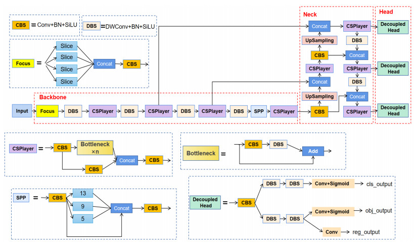
Aerial remote sensing images have complex backgrounds and numerous small targets compared to natural images, so detecting targets in aerial images is more difficult. Resource exploration and urban construction planning need to detect targets quickly and accurately in aerial images. High accuracy is undoubtedly the advantage for detection models in target detection. However, high accuracy often means more complex models with larger computational and parametric quantities. Lightweight models are fast to detect, but detection accuracy is much lower than conventional models. It is challenging to balance the accuracy and speed of the model in remote sensing image detection. In this paper, we proposed a new YOLO model. We incorporated the structures of YOLOX-Nano and slim-neck, then used the SPPF module and SIoU function. In addition, we designed a new upsampling paradigm that combined linear interpolation and attention mechanism, which can effectively improve the model's accuracy. Compared with the original YOLOX-Nano, our model had better accuracy and speed balance while maintaining the model's lightweight. The experimental results showed that our model achieved high accuracy and speed on NWPU VHR-10, RSOD, TGRS-HRRSD and DOTA datasets.
Citation: Lei Yang, Guowu Yuan, Hao Wu, Wenhua Qian. An ultra-lightweight detector with high accuracy and speed for aerial images[J]. Mathematical Biosciences and Engineering, 2023, 20(8): 13947-13973. doi: 10.3934/mbe.2023621
Aerial remote sensing images have complex backgrounds and numerous small targets compared to natural images, so detecting targets in aerial images is more difficult. Resource exploration and urban construction planning need to detect targets quickly and accurately in aerial images. High accuracy is undoubtedly the advantage for detection models in target detection. However, high accuracy often means more complex models with larger computational and parametric quantities. Lightweight models are fast to detect, but detection accuracy is much lower than conventional models. It is challenging to balance the accuracy and speed of the model in remote sensing image detection. In this paper, we proposed a new YOLO model. We incorporated the structures of YOLOX-Nano and slim-neck, then used the SPPF module and SIoU function. In addition, we designed a new upsampling paradigm that combined linear interpolation and attention mechanism, which can effectively improve the model's accuracy. Compared with the original YOLOX-Nano, our model had better accuracy and speed balance while maintaining the model's lightweight. The experimental results showed that our model achieved high accuracy and speed on NWPU VHR-10, RSOD, TGRS-HRRSD and DOTA datasets.

| [1] |
M. Lu, Y. Xu, H. Li, Vehicle Re-Identification based on UAV viewpoint: dataset and method, Remote Sens., 14 (2022), 4630. https://doi.org/10.3390/rs14184603 doi: 10.3390/rs14184603

|
| [2] |
S. Ijlil, A. Essahlaoui, M. Mohajane, N. Essahlaoui, E. M. Mili, A. V. Rompaey, Machine learning algorithms for modeling and mapping of groundwater pollution risk: A study to reach water security and sustainable development (Sdg) goals in a editerranean aquifer system, Remote Sens., 14 (2022), 2379. https://doi.org/10.3390/rs14102379 doi: 10.3390/rs14102379
|
| [3] |
Z. Jiang, Z. Song, Y. Bai, X. He, S. Yu, S. Zhang, et al., Remote sensing of global sea surface pH based on massive underway data and machine mearning, Remote Sens., 14 (2022), 2366. https://doi.org/10.3390/rs14102366 doi: 10.3390/rs14102366
|
| [4] |
Y. Zhao, L. Ge, H. Xie, G. Bai, Z. Zhang, Q. Wei, et al., ASTF: Visual abstractions of time-varying patterns in radio signals, IEEE Trans. Visual Comput. Graphics, 29 (2023), 214–224. https://doi.org/10.1109/TVCG.2022.3209469 doi: 10.1109/TVCG.2022.3209469
|
| [5] | R. Girshick, J. Donahue, T. Darrell J. Malik, Rich feature hierarchies for accurate object detection and semantic segmentation, in 2014 IEEE Conference on Computer Vision and Pattern Recognition (CVPR), (2014), 580–587. https://doi.org/10.1109/CVPR.2014.81 |
| [6] | R. Girshick, Fast R-CNN, in 2015 IEEE International Conference on Computer Vision (ICCV), (2015), 1440–1448. https://doi.org/10.1109/ICCV.2015.169 |
| [7] |
S. Ren, K. He, R. Girshick, J. Sun, Faster R-CNN: Towards real-time object detection with region proposal networks, IEEE Trans. Pattern Anal. Mach. Intell., 39 (2017), 1137–1149. https://doi.org/10.1109/TPAMI.2016.2577031 doi: 10.1109/TPAMI.2016.2577031
|
| [8] | J. Redmon, S. Divvala, R. Girshick, A. Farhadi, You only look once: Unified, real-time object detection, in 2016 IEEE Conference on Computer Vision and Pattern Recognition (CVPR), (2016), 779–788. https://doi.org/10.1109/CVPR.2016.91 |
| [9] | J. Redmon, A. Farhadi, YOLO9000: Better, Faster, Stronger, in 2017 IEEE Conference on Computer Vision and Pattern Recognition (CVPR), (2017), 6517–6525. https://doi.org/10.1109/CVPR.2017.690 |
| [10] | J. Redmon, A. Farhadi, YOLOv3: an incremental improvement, arXiv preprint, (2018), arXiv: 1804.02767. http://arXiv.org/abs/1804.02767 |
| [11] | A. Bochkovskiy, C. Y. Wang, H. Liao, YOLOv4: optimal speed and accuracy of object detection, arXiv preprint, (2020), arXiv: 2004.10934. http://arXiv.org/abs/2004.10934 |
| [12] | G. Jocher, Yolov5, 2020. Available from: https://github.com/ultralytics/yolov5. |
| [13] | Z. Ge, S. Liu, F. Wang, Z. Li, J. Sun, YOLOX: Exceeding YOLO series in 2021, arXiv preprint, (2021), arXiv: 2107.08430. https://arXiv.org/abs/2107.08430 |
| [14] |
Y. Li, X. Liu, H. Zhang, X. Li, X. Sun, Optical remote sensing image retrieval based on convolutional neural networks (in Chinese), Opt. Precis. Eng., 26 (2018), 200–207. https://doi.org/10.3788/ope.20182601.0200 doi: 10.3788/ope.20182601.0200
|
| [15] | A. Van Etten, You only look twice: Rapid multi-scale object detection in satellite imagery, arXiv preprint, (2018), arXiv: 1805.09512. https://doi.org/10.48550/arXiv.1805.09512 |
| [16] |
M. Ahmed, Y. Wang, A. Maher, X. Bai, Fused RetinaNet for small target detection in aerial images, Int. J. Remote Sens., 43 (2022), 2813–2836. https://doi.org/10.1080/01431161.2022.2071115 doi: 10.1080/01431161.2022.2071115
|
| [17] |
H. Liu, G. Yuan, L. Yang, K. Liu, H. Zhou, An appearance defect detection method for cigarettes based on C‐CenterNet, Electronics, 11 (2022), 2182. https://doi.org/10.3390/electronics11142182 doi: 10.3390/electronics11142182
|
| [18] |
S. Du, B. Zhang, P. Zhang, P. Xiang, H. Xue, FA-YOLO: An improved YOLO model for infrared occlusion object detection under confusing background, Wireless Commun. Mobile Comput., 2021 (2021). https://doi.org/10.1155/2021/1896029 doi: 10.1155/2021/1896029
|
| [19] | A. G. Howard, M. Zhu, B. Chen, D. Kalenichenko, W. Wang, T. Weyand, et al., MobileNets: Efficient convolutional neural networks for mobile vision applications, arXiv preprint, (2017), arXiv: 1704.04861. https://doi.org/10.48550/arXiv.1704.04861 |
| [20] | M. Sandler, A. Howard, M. Zhu, A. Zhmoginov, L. C. Chen, MobileNetV2: Inverted residuals and linear bottlenecks, in 2018 IEEE/CVF Conference on Computer Vision and Pattern Recognition (CVPR), (2018), 4510–4520. https://doi.org/10.1109/CVPR.2018.00474 |
| [21] | A. Howard, M. Sandler, B. Chen, W. Wang, L. C. Chen, M. Tan, et al., Searching for mobileNetV3, in 2019 IEEE/CVF International Conference on Computer Vision (ICCV), (2019), 1314–1324. https://doi.org/10.1109/ICCV.2019.00140 |
| [22] | X. Zhang, X. Zhou, M. Lin, J. Sun, ShuffleNet: An extremely efficient convolutional neural network for mobile devices, in Proceedings of the IEEE Conference on Computer Vision and Pattern Recognition (CVPR), (2018), 6848–6856. |
| [23] | N. Ma, X. Zhang, H. T. Zheng, J. Sun, ShuffleNet V2: Practical guidelines for efficient CNN architecture design, in European Conference on Computer Vision (ECCV), (2018), 122–138. https://doi.org/10.1109/CVPR.2018.00716 |
| [24] | RangiLyu, NanoDet-Plus: Super fast and high accuracy lightweight anchor-free object detection model, 2021. Available from: https://github.com/RangiLyu/nanodet. |
| [25] | C. Y. Wang, H. Liao, Y. H. Wu, P. Y. Chen, J. W. Hsieh, I. H. Yeh, CSPNet: A bew backbone that can enhance learning capability of CNN, in 2020 IEEE/CVF Conference on Computer Vision and Pattern Recognition Workshops (CVPRW), (2020), 1571–1580. https://doi.org/10.1109/CVPRW50498.2020.00203 |
| [26] |
X. Luo, Y. Wu, L. Zhao, YOLOD: A target detection method for UAV aerial imagery, Remote Sens., 14 (2022), 3240. https://doi.org/10.3390/rs14143240 doi: 10.3390/rs14143240
|
| [27] |
D. Yan, G. Li, X. Li, H. Zhang, H. Lei, K. Lu, et al., An improved faster R-CNN method to detect tailings ponds from high-resolution remote sensing images, Remote Sens. 13 (2021), 2052. https://doi.org/10.3390/rs13112052 doi: 10.3390/rs13112052
|
| [28] | F. C. Akyon, S. O. Altinuc, A. Temizel, Slicing aided hyper inference and fine-tuning for small object detection, in 2022 IEEE International Conference on Image Processing (ICIP), (2022), 966–970. https://doi.org/10.1109/ICIP46576.2022.9897990 |
| [29] |
L. Yang, G. Yuan, H. Zhou, H. Liu, J. Chen, H. Wu, RS-YOLOX: A high-precision detector for object detection in satellite remote sensing images, Appli. Sci., 12 (2022), 8707. https://doi.org/10.3390/app12178707 doi: 10.3390/app12178707
|
| [30] |
J. Liu, C. Liu, Y. Wu, Z. Sun, H. Xu, Insulators' identification and missing defect detection in aerial images based on cascaded YOLO models, Comput. Intell. Neurosci., 2022 (2022). https://doi.org/10.1155/2022/7113765 doi: 10.1155/2022/7113765
|
| [31] | X. Li, Y. Qin, F. Wang, F. Guo, J. T. W. Yeow, Pitaya detection in orchards using the MobileNet-YOLO model, in 2020 39th Chinese Control Conference (CCC), (2020), 6274–6278. https://doi.org/10.23919/CCC50068.2020.9189186 |
| [32] | Z. Tian, C. Shen, H. Chen, T. He, FCOS: Fully convolutional one-stage object detection, in 2019 IEEE/CVF International Conference on Computer Vision (ICCV), (2019), 9626–9635. https://doi.org/10.1109/ICCV.2019.00972 |
| [33] |
H. Law, J. Deng, CornerNet: Detecting objects as paired keypoints, Int. J. Comput. Vision, 128 (2020), 642–656. https://doi.org/10.1007/s11263-019-01204-1 doi: 10.1007/s11263-019-01204-1
|
| [34] | G. Song, Y. Liu, X. Wang, Revisiting the sibling head in object detector, in Proceedings of the IEEE/CVF Conference on Computer Vision and Pattern Recognition (CVPR), (2020), 11563–11572. |
| [35] |
K. He, X. Zhang, S. Ren, J. Sun, Spatial pyramid pooling in deep convolutional networks for visual recognition, IEEE Trans. Pattern Anal. Mach. Intell., 37 (2015), 1904–1916. https://doi.org/10.1109/TPAMI.2015.2389824 doi: 10.1109/TPAMI.2015.2389824
|
| [36] |
L. C. Chen, G. Papandreou, I. Kokkinos, K. Murphy, A. L. Yuille, DeepLab: Semantic image segmentation with deep convolutional nets, atrous convolution, and fully connected CRFs, IEEE Trans. Pattern Anal. Mach. Intell., 40 (2018), 834–848. https://doi.org/10.1109/TPAMI.2017.2699184 doi: 10.1109/TPAMI.2017.2699184
|
| [37] | C. Y. Wang, A. Bochkovskiy, H. Liao, YOLOv7: Trainable bag-of-freebies sets new state-of-the-art for real-time object detectors, in Proceedings of the IEEE/CVF Conference on Computer Vision and Pattern Recognition (CVPR), (2023), 7464–7475. |
| [38] | H. Li, J. Li, H. Wei, Z. Liu, Z. Zhan, Q. Ren, Slim-neck by GSConv: A better design paradigm of detector architectures for autonomous vehicles, arXiv preprint, (2022), arXiv: 2206.02424. https://doi.org/10.48550/arXiv.2206.02424 |
| [39] | V. Dumoulin, F. Visin, A guide to convolution arithmetic for deep learning, arXiv preprint, (2018), arXiv: 1603.07285. https://doi.org/10.48550/arXiv.1603.07285 |
| [40] | F. Yu, V. Koltun, T. Funkhouser, Dilated residual networks, in 2017 IEEE Conference on Computer Vision and Pattern Recognition (CVPR), (2017), 636–644. https://doi.org/10.1109/CVPR.2017.75 |
| [41] | Q. Wang, B. Wu, P. Zhu, P. Li, W. Zuo, Q. Hu, ECA-Net: Efficient channel attention for deep convolutional neural networks, in 2020 IEEE/CVF Conference on Computer Vision and Pattern Recognition (CVPR), (2020), 11531–11539. https://doi.org/10.1109/CVPR42600.2020.01155 |
| [42] | B. Jiang, R. Luo, J. Mao, T. Xiao, Y. Jiang, Acquisition of localization confidence for accurate object detection, in Proceedings of the European Conference on Computer Vision (ECCV), (2018), 784–799. |
| [43] | J. He, S. Erfani, X. Ma, J. Bailey, Y. Chi, X. S. Hua, Alpha-IoU: A family of power intersection over union losses for bounding box regression, in NeurIPS 2021 Conference, 2021. |
| [44] | H. Rezatofighi, N. Tsoi, J. Gwak, A. Sadeghian, I. Reid, S. Savarese, Generalized intersection over union: A metric and a loss for bounding box regression, in 2019 IEEE/CVF Conference on Computer Vision and Pattern Recognition (CVPR), (2019), 658–666. https://doi.org/10.1109/CVPR.2019.00075 |
| [45] | Z. Zheng, P. Wang, W. Liu, J. Li, R. Ye, D. Ren, Distance-IoU loss: Faster and better learning for bounding box regression, in Proceedings of the AAAI Conference on Artificial Intelligence, 2020. https://doi.org/10.1609/aaai.v34i07.6999 |
| [46] | Z. Gevorgyan, SIoU loss: More powerful learning for bounding box regression, arXiv preprint, (2022), arXiv: 2205.12740. https://doi.org/10.48550/arXiv.2205.12740 |
| [47] |
G. Cheng, P. Zhou, J. Han, Learning rotation-invariant convolutional neural networks for object detection in VHR optical remote sensing images, IEEE Trans. Geosci. Remote Sens., 54 (2016), 7405–7415. https://doi.org/10.1109/TGRS.2016.2601622 doi: 10.1109/TGRS.2016.2601622
|
| [48] |
Y. Long, Y. Gong, Z. Xiao, Q. Liu, Accurate object localization in remote sensing images based on convolutional neural networks, IEEE Trans. Geosci. Remote Sens., 55 (2017), 2486–2498. https://doi.org/10.1109/TGRS.2016.2645610 doi: 10.1109/TGRS.2016.2645610
|
| [49] |
X. Lu, Y. Zhang, Y. Yuan, Y. Feng, Gated and axis-concentrated localization network for remote sensing object detection, IEEE Trans. Geosci. Remote Sens., 58 (2020), 179–192. https://doi.org/10.1109/TGRS.2019.2935177 doi: 10.1109/TGRS.2019.2935177
|
| [50] | L. Yang, R. Y. Zhang, L. Li, X. Xie, SimAM: A simple, parameter-free attention module for convolutional neural networks, in Proceedings of the 38th International Conference on Machine Learning, 139 (2021), 11863–11874. |
| [51] | Z. Zhong, Z. Q. Lin, R. Bidart, X. Hu, I. B. Daya, Z. Li, et al., Squeeze-and-attention networks for semantic segmentatio, in Proceedings of the IEEE/CVF Conference on Computer Vision and Pattern Recognition (CVPR), (2020), 13065–13074. |
| [52] | R. Saini, N. K. Jha, B. Das, S. Mittal, C. K. Mohan, ULSAM: Ultra-lightweight subspace attention module for compact convolutional neural networks, in Proceedings of the IEEE/CVF Winter Conference on Applications of Computer Vision (WACV), (2020), 1616–1625. https://doi.org/10.1109/WACV45572.2020.9093341 |
| [53] | Y. Liu, Z. Shao, Y. Teng, N. Hoffmann, NAM: Normalization-based attention module, arXiv preprint, (2021), arXiv: 2111.12419. https://doi.org/10.48550/arXiv.2111.12419 |
| [54] | X. Ma, Yolo-Fastest: yolo-fastest-v1.1.0, 2021. Available from: https://github.com/dog-qiuqiu/Yolo-Fastest. |
| [55] | X. Ma, FastestDet: Ultra lightweight anchor-free real-time object detection algorithm, 2022. Available from: https://github.com/dog-qiuqiu/FastestDet. |
| [56] | X. Yang, J. Yan, Z. Feng, T. He, R3Det: Refined single-stage detector with feature refinement for rotating object, in Proceedings of the AAAI Conference on Artificial Intelligence, 35 (2021), 3163–3173. https://doi.org/10.1609/aaai.v35i4.16426 |
| [57] |
J. Han, J. Ding, J. Li, G. S. Xia, Align deep features for oriented object detection, IEEE Trans. Geosci. Remote Sens., 60 (2022), 1–11. https://doi.org/10.1109/TGRS.2021.3062048 doi: 10.1109/TGRS.2021.3062048
|
| [58] | X. Xie, G. Cheng, J. Wang, X. Yao, J. Han, Oriented R-CNN for object detection, in 2021 IEEE/CVF International Conference on Computer Vision (ICCV), (2021), 3500–3509. https://doi.org/10.1109/ICCV48922.2021.00350 |
| [59] | J. Ding, N. Xue, Y. Long, G. S. Xia, Q. Lu, Learning RoI transformer for oriented object detection in aerial images, in 2019 IEEE/CVF Conference on Computer Vision and Pattern Recognition (CVPR), (2019), 2844–2853. https://doi.org/10.1109/CVPR.2019.00296 |
| [60] |
S. Zhong, H. Zhou, Z. Ma, F. Zhang, J. Duan, Multiscale contrast enhancement method for small infrared target detection, Optik, 271 (2022), 170134. https://doi.org/10.1016/j.ijleo.2022.170134 doi: 10.1016/j.ijleo.2022.170134
|
| [61] |
S. Zhong, H. Zhou, X. Cui, X. Cao, F. Zhang, J. Duan, Infrared small target detection based on local-image construction and maximum correntropy, Measurement, 211 (2023), 112662. https://doi.org/10.1016/j.measurement.2023.112662 doi: 10.1016/j.measurement.2023.112662
|


Figures(16) / Tables(11)

Lei Yang, Guowu Yuan, Hao Wu, Wenhua Qian. An ultra-lightweight detector with high accuracy and speed for aerial images[J]. Mathematical Biosciences and Engineering, 2023, 20(8): 13947-13973. doi: 10.3934/mbe.2023621


 DownLoad: