Controlling malaria in a population accessing counterfeit antimalarial drugs

Baaba A. Danquah; Faraimunashe Chirove; Jacek Banasiak; Baaba A. Danquah; Faraimunashe Chirove; Jacek Banasiak

doi:10.3934/mbe.2023529

Mathematical Biosciences and Engineering

2023, Volume 20, Issue 7: 11895-11938. doi: 10.3934/mbe.2023529

Previous Article Next Article

Research article Special Issues

Controlling malaria in a population accessing counterfeit antimalarial drugs

1.
Department of Mathematics and Statistics, University of Energy and Natural Resources, P. O. Box 214, Sunyani, Ghana
2.
Department of Mathematics, University of Johannesburg, Johannesburg, South Africa
3.
School of Mathematics and Applied Mathematics, University of Pretoria, Pretoria, South Africa
4.
Institute of Mathematics, Łódź University of Technology, Łódź, Poland

Academic Editor: Wandi Ding

Received: 01 December 2022 Revised: 15 March 2023 Accepted: 28 March 2023 Published: 10 May 2023

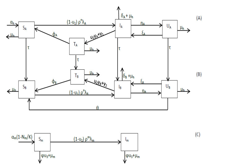
A mathematical model is developed for describing malaria transmission in a population consisting of infants and adults and in which there are users of counterfeit antimalarial drugs. Three distinct control mechanisms, namely, effective malarial drugs for treatment and insecticide-treated bednets (ITNs) and indoor residual spraying (IRS) for prevention, are incorporated in the model which is then analyzed to gain an understanding of the disease dynamics in the population and to identify the optimal control strategy. We show that the basic reproduction number, $ R_{0} $, is a decreasing function of all three controls and that a locally asymptotically stable disease-free equilibrium exists when $ R_{0} < 1 $. Moreover, under certain circumstances, the model exhibits backward bifurcation. The results we establish support a multi-control strategy in which either a combination of ITNs, IRS and highly effective drugs or a combination of IRS and highly effective drugs is used as the optimal strategy for controlling and eliminating malaria. In addition, our analysis indicates that the control strategies primarily benefit the infant population and further reveals that a high use of counterfeit drugs and low recrudescence can compromise the optimal strategy.
- malaria,
- structured population,
- reproduction numbers,
- backward bifurcation,
- optimal control,
- counterfeit drugs
Citation: Baaba A. Danquah, Faraimunashe Chirove, Jacek Banasiak. Controlling malaria in a population accessing counterfeit antimalarial drugs[J]. Mathematical Biosciences and Engineering, 2023, 20(7): 11895-11938. doi: 10.3934/mbe.2023529

Related Papers:

Abstract

A mathematical model is developed for describing malaria transmission in a population consisting of infants and adults and in which there are users of counterfeit antimalarial drugs. Three distinct control mechanisms, namely, effective malarial drugs for treatment and insecticide-treated bednets (ITNs) and indoor residual spraying (IRS) for prevention, are incorporated in the model which is then analyzed to gain an understanding of the disease dynamics in the population and to identify the optimal control strategy. We show that the basic reproduction number, $ R_{0} $, is a decreasing function of all three controls and that a locally asymptotically stable disease-free equilibrium exists when $ R_{0} < 1 $. Moreover, under certain circumstances, the model exhibits backward bifurcation. The results we establish support a multi-control strategy in which either a combination of ITNs, IRS and highly effective drugs or a combination of IRS and highly effective drugs is used as the optimal strategy for controlling and eliminating malaria. In addition, our analysis indicates that the control strategies primarily benefit the infant population and further reveals that a high use of counterfeit drugs and low recrudescence can compromise the optimal strategy.

References

[1]	World Health Organization, Neglected tropical diseases, mosquito borne-diseases, World Health Organization (Geneva-Switzerland, 2015).
[2]	World Health Organization, World Malaria Report 2021, World Health Organization (Geneva-Switzerland, 2021). Available from: http://www.who.int/malaria/publications/world-malaria-report-2021/report/en/.
[3]	D. L. Doolan, C. Dobano, J. Y. Baird, Acquired immunity to malaria, Clinical Microbiology Review, 22 (2009), 13–36. https://journals.asm.org/doi/10.1128/CMR.00025-08 doi: 10.1128/CMR.00025-08
[4]	World Health Organization, World Malaria Report 2017, World Health Organization (Geneva-Switzerland, 2017). Available from: http://www.who.int/malaria/publications/world-malaria-report-2017/report/en/.
[5]	World Health Organization, World Malaria Report 2015, World Health Organization (Geneva-Switzerland, 2015). Available from: http://www.who.int/malaria/publications/world-malaria-report-2015/report/en/.
[6]	Global Malaria Programme, Malaria Prevention Works - let's close the gap, World Health Organization (Geneva-Switzerland, 2017). Available from: http://www.who.int/malaria.
[7]	World Health Organization, Guidelines for the treatment of malaria-3rd edition, World Health Organization (Geneva-Switzerland, 2015).
[8]	W. Ittarat, A. L. Pickard, P. Rattanasinganchan, P. Wilairatana, S. Looareesuwan, K. Emery, et al., Recrudescence in artesunate-treated patients with falciparum malaria is dependent on parasite burden not on parasite factors, Am. Soc. Trop. Med. Hyg., 68 (2003), 147–152.
[9]	K. A. Koram, B. Abuaku, N. Duah, N. Quashie, Comparative efficacy of antimalarial drugs including ACTs in the treatment of uncomplicated malaria among children under 5 years in Ghana, Acta Trop., 95 (2005), 195–203. https://doi.org/10.1016/j.actatropica.2005.06.018 doi: 10.1016/j.actatropica.2005.06.018
[10]	R. Bate, Making a Killing: The Deadly Implication of the Counterfeit Drug Trade, AEI Press, Washington DC, 2008.
[11]	K. O. Buabeng, M. Duwiejua, L. K. Matowe, F. Smith, H. Enlund, Availability and choice of antimalarials at medicine outlets in Ghana: the question of access to effective medicines for malaria control, Clin. Pharmacol. Ther., 84 (2008), 613–619. https://doi.org/10.1038/clpt.2008.130 doi: 10.1038/clpt.2008.130
[12]	G. M. L. Nayyar, J. G. Breman, P. N. Newton, J. Herrington, Poor-quality antimalarial drugs in southeast Asia and Sub-Saharan Africa, Lancet Infect. Dis., 12 (2012), 488–496. https://doi.org/10.1016/S1473-3099(12)70064-6 doi: 10.1016/S1473-3099(12)70064-6
[13]	P. N. Newton, M. D. Green, D. C. Mildenhall, A. Plancon, H. Nettey, L. Nyadong, et al., Poor quality vital antimalarials in Africa–an urgent neglected public health priority, Malaria J., 10 (2011), 352. https://doi.org/10.1186/1475-2875-10-352 doi: 10.1186/1475-2875-10-352
[14]	K. A. O'Connell, H. Gatakaa, S. Poyer, J. Njogu, I. Evance, E. Munroe, et al., Got ACTs? Availability, price, market share and provider knowledge of antimalarial medicines in public and private sector outlets in six malaria-endemic countries, Malaria J., 10 (2011), 326. https://doi.org/10.1186/1475-2875-10-326 doi: 10.1186/1475-2875-10-326
[15]	J. P. Renschler, K. M. Walters, P. N. Newton, R. Laxminarayan, Estimated under-five deaths associated with poor-quality antimalarials in Sub-Saharan Africa, Am. J. Trop. Med. Hyg., 92 (2015), 119–126. https://doi.org/10.4269/ajtmh.14-0725 doi: 10.4269/ajtmh.14-0725
[16]	C. Sayang, M. Gausseres, N. Vernazza-Licht, D. Malvy, D. Blay, P. Millet, Treatment of malaria from monotherapy to artemisinin-based combination therapy by health professionals in rural health facilities in southern Cameroon, Malaria J., 8 (2009), 174. https://doi.org/10.1186/1475-2875-8-176 doi: 10.1186/1475-2875-8-176
[17]	Centers for Disease Control and Prevention, Counterfeit and substandard antimalarial drugs. Available from: https://www.cdc.gov/malaria/malaria-worldwide/reduction/counterfeit.html.
[18]	P. B. Bloland, Drug Resistance in Malaria, World Health Organization, Switzerland, 2001. Available from: http://www.who.int/csr/resources/publications/drugresist/malaria.pdf.
[19]	C. Chiyaka, W. Garira, S. Dube, Effect of treatment and drug resistance on the transmission dynamics of malaria in endemic areas, Theor. Popul. Biol., 75 (2009), 14–29. https://doi.org/10.1016/j.tpb.2008.10.002 doi: 10.1016/j.tpb.2008.10.002
[20]	C. Chiyaka, J. M. Tchuenche, W. Garira, S. Dube, A mathematical analysis of the effects of control strategies on the transmission dynamics of Malaria, Appl. Math. Comput., 195 (2008), 641–662. https://doi.org/10.1016/j.amc.2007.05.016 doi: 10.1016/j.amc.2007.05.016
[21]	F. Forouzannia, A. B. Gumel, Mathematical analysis of an age-structured model for malaria transmission dynamics, Math. Biosci., 247 (2014), 80–94. https://doi.org/10.1016/j.mbs.2013.10.011 doi: 10.1016/j.mbs.2013.10.011
[22]	F. Forouzannia, A. B. Gumel, Dynamics of an age-structured two-strain model for malaria transmission, Appl. Math. Comput., 250 (2015), 860–886. https://doi.org/10.1016/j.amc.2014.09.117 doi: 10.1016/j.amc.2014.09.117
[23]	K. O. Okosun, R. Ouifki, N. Marcus, Optimal control strategies and cost-effectiveness analysis of a malaria model, Biosystems, 111 (2013), 83–101. https://doi.org/10.1016/j.biosystems.2012.09.008 doi: 10.1016/j.biosystems.2012.09.008
[24]	F. B. Agusto, N. Marcus, K. O. Okosun, Application of optimal control to the epidemiology of malaria, Electron. J. Differ. Equations, 81 (2012), 1–22.
[25]	N. R. Chitnis, Using mathematical models in controlling the spread of malaria, (PhD thesis, The University of Arizona, Arizona, 2005).
[26]	C. Chiyaka, W. Garira, S. Dube, Transmission model of endemic human malaria in a partially immune population, Math. Comput. Model., 46 (2007), 806–822. https://doi.org/10.1016/j.mcm.2006.12.010 doi: 10.1016/j.mcm.2006.12.010
[27]	H. F. Huo and G. M. Qui, Stability of a mathematical model of malaria transmission with relapse, Abstr. Appl. Anal., 2014 (2014), 9. https://doi.org/10.1155/2014/289349 doi: 10.1155/2014/289349
[28]	G. A. Ngwa, W. S. Shu, A mathematical model for endemic malaria with variable human and mosquito populations, Math. Comput. Model., 32 (2000), 747–763. https://doi.org/10.1016/S0895-7177(00)00169-2 doi: 10.1016/S0895-7177(00)00169-2
[29]	M. N. Ashrafi, B. A. Gumel, Mathematical analysis of the role of repeated exposure on malaria transmission dynamics, Differ. Equations Dyn. Syst., 16 (2008), 251–287. https://doi.org/10.1007/s12591-008-0015-1 doi: 10.1007/s12591-008-0015-1
[30]	L. Cai, A. A. Lashari, I. H. Jung, K. O. Okosun, Y. I. Seo, Mathematical analysis of a malaria model with partial immunity to reinfection, Abstr. Appl. Anal., 2013 (2013), 17. https://doi.org/10.1155/2013/405258 doi: 10.1155/2013/405258
[31]	J. M. Addawe, J. E. Lope, Analysis of an age-structured malaria transmission model, Philipp. Sci. Lett., 5 (2012), 162–182.
[32]	J. Wairimu, S. Gauthier, W. Ogana, Formulation of a vector SIS malaria model in a patchy environment with two age classes, Appl. Math., 5 (2014), 1535–1545. https://doi.org/10.4236/am.2014.510147 doi: 10.4236/am.2014.510147
[33]	J. Arino, A. Ducrot, P. Zongo, A metapopulation model for malaria with transmission-blocking partial immunity in hosts, J. Math. Biol., 64 (2012), 423–448. https://doi.org/10.1007/s00285-011-0418-4 doi: 10.1007/s00285-011-0418-4
[34]	L. S. Pontryagin, V. G. Boltyanskii, R. V. Gamkrelidze, E. F. Mishchenko, The Mathematical Theory of Optimal Processes, Wiley, New York, 1962.
[35]	K. Blayneh, Y. Cao, H. D. Kwon, Optimal control of vector-borne disease: Treatment and prevention, Discrete Continuous Dyn. Syst. Ser. B, 11 (2009), 587–611. https://doi.org/10.3934/DCDSB.2009.11.587 doi: 10.3934/DCDSB.2009.11.587
[36]	K. O. Okosun, O. D. Makinde, Optimal control analysis of malaria in the presence of non-linear incidence rate, Appl. Comput. Math., 12 (2013), 20–32.
[37]	K. O. Okosun, R. Smith, Optimal control analysis of malaria-schistosomiasis co-infection dynamics, Math. Biosci. Eng., 14 (2017), 377–405. https://doi.org/10.3934/mbe.2017024 doi: 10.3934/mbe.2017024
[38]	M. Rafikov, L. Bevilacqua, A. P. P. Wyse, Optimal control strategy of malaria vector using genetically modified mosquitoes, J. Theor. Biol., 258 (2009), 418–425. https://doi.org/10.1016/j.jtbi.2008.08.006 doi: 10.1016/j.jtbi.2008.08.006
[39]	H. Kwon, J. Lee, D. Yang, Optimal control of an age-structured model of HIV infection, Appl. Math. Comput., 219 (2012), 2766–2779. https://doi.org/10.1016/j.amc.2012.09.003 doi: 10.1016/j.amc.2012.09.003
[40]	Ghana Statistical Service, Ghana Multiple Indicator Cluster Survey with an Enhanced Malaria Module and Biomarker 2011 Final Report, Ghana Statistical Service, (Accra, Ghana, 2011).
[41]	D. Moulay, M. A. Aziz-Alaoui, H. Kwon, Optimal control of chikungunya disease: larvae reduction, treatment and prevention, Math. Biosci. Eng., 9 (2012), 369–393.
[42]	K. Dietz, L. Molineaux, A. Thomas, A malaria model tested in the African savannah, Bull. World Health Organ., 50 (1974), 347–357.
[43]	H. W. Hethcote, The Mathematics of Infectious disease, SIAM Rev. Soc. Ind. Appl. Math., 42 (2000), 599–653. https://doi.org/10.1137/S0036144500371907 doi: 10.1137/S0036144500371907
[44]	W. P. O'Meara, D. L. Smith, F. E. McKenzie, Potential impact of intermittent preventive treatment (IPT) on spread of drug-resistant malaria, PLoS Med., 3 (2006). https://doi.org/10.1371/journal.pmed.0030141 doi: 10.1371/journal.pmed.0030141
[45]	B. A. Danquah, F. Chirove, J. Banasiak, Effective and ineffective treatment in a malaria model for humans in an endemic area, Afrika Math., 30 (2019), 1181–1204. https://doi.org/10.1007/s13370-019-00713-z doi: 10.1007/s13370-019-00713-z
[46]	P. van den Driessche, J. Watmough, Reproduction numbers and sub-threshold endemic equilibria for compartmental models of disease transmission, Math. Biosci., 180 (2002), 29–48. https://doi.org/10.1016/S0025-5564(02)00108-6 doi: 10.1016/S0025-5564(02)00108-6
[47]	C. Castillo–Chavez, B. Song, Dynamical models of tuberculosis and their applications, Math. Biosci. Eng., 1 (2004), 361–404.
[48]	A. R. Oduro, T. Anyorigiya, A. Hodgson, P. Ansah, F. Anto, A. N. Ansah, et al., A randomized comparative study of chloroquine, amodiaquine and sulphadoxine-pyrimethamine for the treatment of uncomplicated malaria in Ghana, Trop. Med. Int. Health, 3 (2005), 279–284. https://doi.org/10.1111/j.1365-3156.2004.01382.x doi: 10.1111/j.1365-3156.2004.01382.x
[49]	D. L. Lukes, Differential Equations: Classical to Controlled, Academic Press, New York, 1982.
[50]	W. H. Fleming, R. W. Rishel, Deterministic and Stochastic Optimal Control, Springer Verlag, New York, 1975.
[51]	S. Lenhart, J. T. Workman, Control Applied to Biological Models, Chapman and Hall, London, 2007.
[52]	K. Badu, C. Brenya, C. Timmann, R. Garms, T. F. Kruppa, Malaria transmission intensity and dynamics of clinical malaria incidence in a mountainous forest region of Ghana, Malaria World J., 4 (2013), 14.
[53]	S. Kasasa, V. Asoala, L. Gosoniu, F. Anto, M. Adjuik, C. Tindana, et al., Spatio-temporal malaria transmission patterns in Navrongo demographic surveillance site, Northern Ghana, Malaria J., 12 (2013), 63. https://doi.org/10.1186/1475-2875-12-63 doi: 10.1186/1475-2875-12-63
[54]	S. C. K. Tay, S. K. Danuor, D. C. Mensah, G. Acheampong, H. H. Abuquah, A. Morse, et al., Climate variability and malaria incidence in peri-urban, urban and rural communities around Kumasi, Ghana: a case study at three health facilities; Emena, Atonsu and Akropong, Int. J. Parasitology Res., 4 (2012), 83–89.
[55]	D. Tchouassi, I. A. Quakyi, E. A. Addison, K. M. Bosompem, M. D. Wilson, M. A. Appawu, et al., Characterization of malaria transmission by vector populations for improved interventions during the dry season in the Kpone-on-Sea area of coastal Ghana, Parasites Vectors, 5 (2012), 212. https://doi.org/10.1186/1756-3305-5-212 doi: 10.1186/1756-3305-5-212
[56]	United Nations Children's Fund, Levels and Trends in Child Mortality, 2014.
[57]	World Health Organization, Ghana: WHO statistical profile, World Health Organization, Geneva-Switzerland, 2017.
[58]	D. S. Rowe, The special programme for research and training in tropical diseases, Critical Rev. Trop. Med., 2 (1984), 1–38. https://doi.org/10.1007/978-1-4613-2723-3_1 doi: 10.1007/978-1-4613-2723-3_1
[59]	A. K. Githeko, J. M. Ayisi, P. K. Odada, F. K. Atieli, B. A. Ndenga, J. I. Githure, et al., Topography and malaria transmission heterogeneity in western Kenya highlands: prospects for focal vector control, Malaria J., 5 (2006). https://doi.org/10.1186/1475-2875-5-107 doi: 10.1186/1475-2875-5-107
[60]	P. E. Parham, E. Michael, Modelling the effects of weather and climate change on malaria transmission, Environ. Health Perspect., 118 (2010), 620–626. https://doi.org/10.1289/ehp.0901256 doi: 10.1289/ehp.0901256

Reader Comments

Your name:*

Email:*
© 2023 the Author(s), licensee AIMS Press. This is an open access article distributed under the terms of the Creative Commons Attribution License (http://creativecommons.org/licenses/by/4.0)