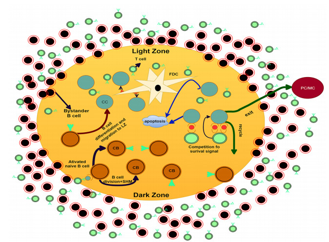
The germinal center (GC) is a self-organizing structure produced in the lymphoid follicle during the T-dependent immune response and is an important component of the humoral immune system. However, the impact of the special structure of GC on antibody production is not clear. According to the latest biological experiments, we establish a spatiotemporal stochastic model to simulate the whole self-organization process of the GC including the appearance of two specific zones: the dark zone (DZ) and the light zone (LZ), the development of which serves to maintain an effective competition among different cells and promote affinity maturation. A phase transition is discovered in this process, which determines the critical GC volume for a successful growth in both the stochastic and the deterministic model. Further increase of the volume does not make much improvement on the performance. It is found that the critical volume is determined by the distance between the activated B cell receptor (BCR) and the target epitope of the antigen in the shape space. The observation is confirmed in both 2D and 3D simulations and explains partly the variability of the observed GC size.
Citation: Zishuo Yan, Hai Qi, Yueheng Lan. The role of geometric features in a germinal center[J]. Mathematical Biosciences and Engineering, 2022, 19(8): 8304-8333. doi: 10.3934/mbe.2022387
The germinal center (GC) is a self-organizing structure produced in the lymphoid follicle during the T-dependent immune response and is an important component of the humoral immune system. However, the impact of the special structure of GC on antibody production is not clear. According to the latest biological experiments, we establish a spatiotemporal stochastic model to simulate the whole self-organization process of the GC including the appearance of two specific zones: the dark zone (DZ) and the light zone (LZ), the development of which serves to maintain an effective competition among different cells and promote affinity maturation. A phase transition is discovered in this process, which determines the critical GC volume for a successful growth in both the stochastic and the deterministic model. Further increase of the volume does not make much improvement on the performance. It is found that the critical volume is determined by the distance between the activated B cell receptor (BCR) and the target epitope of the antigen in the shape space. The observation is confirmed in both 2D and 3D simulations and explains partly the variability of the observed GC size.

| [1] |
A. K. Chakraborty, A. Kosmrlj, Statistical mechanical concepts in immunology, Annu. Rev. Phys. Chem., 61 (2010), 283–303. https://doi.org/10.1146/annurev.physchem.59.032607.093537 doi: 10.1146/annurev.physchem.59.032607.093537

|
| [2] |
P. Nieuwenhuis, D. Opstelten, Functional anatomy of germinal centers, Dev. Dynam., 170 (1984), 421–435. https://doi.org/10.1002/aja.1001700315 doi: 10.1002/aja.1001700315
|
| [3] |
D. M. Tarlinton, K. G. C. Smith, Dissecting affinity maturation: a model explaining selection of antibody-forming cells and memory b cells in the germinal centre, Immunol. Today, 21 (2000), 436–441. https://doi.org/10.1016/S0167-5699(00)01687-X doi: 10.1016/S0167-5699(00)01687-X
|
| [4] | I. C. Maclennan, Germinal centers, Annu. Rev. Immunol., 12 (1994), 117–139. https://doi.org/10.1146/annurev.immunol.12.1.117 |
| [5] |
T. A. Schwickert, R. L. Lindquist, G. Shakhar, G. Livshits, M. C. Nussenzweig, in vivo imaging of germinal centres reveals a dynamic open structure, Nature, 446 (2007), 83–87. https://doi.org/10.1038/nature05573 doi: 10.1038/nature05573
|
| [6] |
Y. Natkunam, The biology of the germinal center, Hematology, 2007 (2007), 210–215. https://doi.org/10.1182/asheducation-2007.1.210 doi: 10.1182/asheducation-2007.1.210
|
| [7] |
C. D. C. Allen, T. Okada, H. Tang, J. G. Cyster, Imaging of germinal center selection events during affinity maturation, Science, 315 (2007), 528–531. https://doi.org/10.1126/science.1136736 doi: 10.1126/science.1136736
|
| [8] | G. D. Victora, M. C. Nussenzweig, Germinal centers, Annu. Rev. Immunol., 30 (2012), 429–457. https://doi.org/10.1146/annurev-immunol-020711-075032 |
| [9] |
A. S. Perelson, G. F. Oster, Theoretical studies of clonal selection: minimal antibody repertoire size and reliability of self-non-self discrimination, J. Theor. Biol., 81 (1979), 645–670. https://doi.org/10.1016/0022-5193(79)90275-3 doi: 10.1016/0022-5193(79)90275-3
|
| [10] |
T. B. Kepler, A. S. Perelson, Cyclic re-entry of germinal center B cells and the efficiency of affinity maturation, Immunol. Today, 14 (1993), 412–415. https://doi.org/10.1016/0167-5699(93)90145-B doi: 10.1016/0167-5699(93)90145-B
|
| [11] |
A. S. Perelson, G. Weisbuch, Immunology for physicists, Rev. Mod. Phys., 69 (1997), 1219–1267. https://doi.org/10.1103/RevModPhys.69.1219 doi: 10.1103/RevModPhys.69.1219
|
| [12] |
M. Oprea, Somatic mutation leads to efficient affinity maturation when centrocytes recycle back to centroblasts, J. Immunol., 158(1997), 5155–5162. https://doi.org/10.1016/S0165-2478(97)85162-0 doi: 10.1016/S0165-2478(97)85162-0
|
| [13] |
S. Erwin, S. M. Ciupe, Germinal center dynamics during acute and chronic infection, Math. Biosci. Eng., 14 (2017), 655–671. https://doi.org/10.3934/mbe.2017037 doi: 10.3934/mbe.2017037
|
| [14] |
M. Meyer-Hermann, M. T. Figge, K. M. Toellner, Germinal centres seen through the mathematical eye: B-cell models on the catwalk, Trends Immunol., 30 (2009), 157–164. https://doi.org/10.1016/j.it.2009.01.005 doi: 10.1016/j.it.2009.01.005
|
| [15] |
L. Buchauer, H. Wardemann, Calculating germinal centre reactions, Curr. Opin. Syst. Biol., 18 (2019), 1–8. https://doi.org/10.1016/j.coisb.2019.10.004 doi: 10.1016/j.coisb.2019.10.004
|
| [16] |
M. J. Shlomchik, F. Weisel, Germinal center selection and the development of memory B and plasma cells, Immunol. Rev., 247 (2012), 52–63. https://doi.org/10.1111/j.1600-065X.2012.01124.x doi: 10.1111/j.1600-065X.2012.01124.x
|
| [17] |
M. Meyer-Hermann, P. K. Maini, Interpreting two-photon imaging data of lymphocyte motility, Phys. Rev. E, 71 (2005), 061912. https://doi.org/10.1103/PhysRevE.71.061912 doi: 10.1103/PhysRevE.71.061912
|
| [18] |
M. T. Figge, A. Garin, M. Gunzer, M. Kosco-Vilbois, K. M. Toellner, M. Meyer-Hermann, Deriving a germinal center lymphocyte migration model from two-photon data, J. Exp. Med., 205 (2008), 3019–3029. https://doi.org/10.1084/jem.20081160 doi: 10.1084/jem.20081160
|
| [19] |
T. Beyer, M. Meyer-Hermann, G. Soff, A possible role of chemotaxis in germinal center formation, Int. Immunol., 14 (2003), 1369–1381. https://doi.org/10.1016/j.celrep.2012.05.010 doi: 10.1016/j.celrep.2012.05.010
|
| [20] |
M. Meyer-Hermann, A mathematical model for the germinal center morphology and affinity maturation, J. Theor. Biol., 216 (2002), 273–300. https://doi.org/10.1016/j.coisb.2019.10.004 doi: 10.1016/j.coisb.2019.10.004
|
| [21] |
M. Meyer-Hermann, A concerted action of b cell selection mechanisms, Adv. Complex. Syst., 10 (2007), 557–580. https://doi.org/10.1142/S0219525907001276 doi: 10.1142/S0219525907001276
|
| [22] |
S. Crotty, T follicular helper cell biology: A decade of discovery and diseases, Immunity, 50 (2019), 1132–1148. https://doi.org/10.1016/j.immuni.2019.04.011 doi: 10.1016/j.immuni.2019.04.011
|
| [23] |
M. Meyer-Hermann, P. K. Maini, A. D. Iber, An analysis of B cell selection mechanisms in germinal centres, Math. Med. Biol., 23 (2006), 255–277. https://doi.org/10.1007/s11538-009-9408-8 doi: 10.1007/s11538-009-9408-8
|
| [24] | M. J. Thomas, U. Klein, J. Lygeros, M. R. Martínez, A probabilistic model of the germinal center reaction, Front. Immunol., 10 (2019). https://doi.org/10.3389/fimmu.2019.00689 |
| [25] |
M. Meyer-Hermann, E. Mohr, N. Pelletier, Y. Zhang, G. D. Victora, K. M. Toellner, A theory of germinal center B cell selection, division, and exit, Cell Rep., 2 (2012), 162–174. https://doi.org/10.1016/j.celrep.2012.05.010 doi: 10.1016/j.celrep.2012.05.010
|
| [26] |
P. A. Robert, A. L. Marschall, M. Meyer-Hermann, Induction of broadly neutralizing antibodies in germinal centre simulations, Curr. Opin. Biotechnol., 51 (2018), 137–145. https://doi.org/10.1016/j.copbio.2018.01.006 doi: 10.1016/j.copbio.2018.01.006
|
| [27] | M. Molari, K. Eyer, J. Baudry, S. Cocco, R. Monasson, Quantitative modeling of the effect of antigen dosage on b-cell affinity distributions in maturating germinal centers, Elife, 9 (2020). https://doi.org/10.7554/elife.55678 |
| [28] | E. M. Tejero, D. Lashgari, R. García-Valiente, X. Gao, F. Crauste, P. A. Robert, et al., Multiscale modeling of germinal center recapitulates the temporal transition from memory B cells to plasma cells differentiation as regulated by antigen affinity-based tfh cell help, Front. Immunol., 11 (2021). https://doi.org/10.3389/fimmu.2020.620716 |
| [29] |
S. Wang, J. Mata-Fink, B. Kriegsman, M. Hanson, D. Irvine, H. Eisen, et al., Manipulating the selection forces during affinity maturation to generate cross-reactive hiv antibodies, Cell, 160 (2015), 785–797. https://doi.org/10.1016/j.cell.2015.01.027 doi: 10.1016/j.cell.2015.01.027
|
| [30] |
N. Wittenbrink, T. S. Weber, A. Klein, A. A. Weiser, W. Zuschratter, M. Sibila, et al., Broad volume distributions indicate nonsynchronized growth and suggest sudden collapses of germinal center B cell populations, J. Immunol., 184 (2010), 1339–1347. https://doi.org/10.4049/jimmunol.0901040 doi: 10.4049/jimmunol.0901040
|
| [31] |
N. Wittenbrink, A. Klein, A. A. Weiser, J. Schuchhardt, M. Or-Guil, Is there a typical germinal center? a large-scale immunohistological study on the cellular composition of germinal centers during the hapten-carrier-driven primary immune response in mice, J. Immunol., 187 (2011), 6185–6196. https://doi.org/10.4049/jimmunol.1101440 doi: 10.4049/jimmunol.1101440
|
| [32] |
P. Wang, C. M. Shih, H. Qi, Y. H. Lan, A stochastic model of the germinal center integrating local antigen competition, individualistic T-B interactions, and B cell receptor signaling, J. Immunol., 197 (2016), 1169–1182. https://doi.org/10.4049/jimmunol.1600411 doi: 10.4049/jimmunol.1600411
|
| [33] |
D. T. Gillespie, Exact stochastic simulation of coupled chemical-reactions, J. Phys. Chem., 81 (1977), 2340–2361. https://doi.org/10.1021/j100540a008 doi: 10.1021/j100540a008
|
| [34] |
A. D. Gitlin, C. T. Mayer, T. Y. Oliveira, Z. Shulman, M. J. K. Jones, A. Koren, et al., T cell help controls the speed of the cell cycle in germinal center B cells, Science, 349 (2015), 643–646. https://doi.org/10.1126/science.aac4919 doi: 10.1126/science.aac4919
|
| [35] |
H. Qi, J. G. Egen, A. Y. C. Huang, R. N. Germain, Extrafollicular activation of lymph node B cells by antigen-bearing dendritic cells, Science, 312 (2006), 1672–1676. https://doi.org/10.1126/science.1125703 doi: 10.1126/science.1125703
|
| [36] |
H. Qi, J. L. Cannons, F. Klauschen, P. L. Schwartzberg, R. N. Germain, Sap-controlled T-B cell interactions underlie germinal centre formation, Nature, 455 (2008), 764–769. https://doi.org/10.1038/nature07345 doi: 10.1038/nature07345
|
| [37] |
J. G. Cyster, Chemokines and cell migration in secondary lymphoid organs, Science, 286 (1999), 2098–2102. https://doi.org/10.1126/science.286.5447.2098 doi: 10.1126/science.286.5447.2098
|
| [38] |
H. Qi, X. Chen, C. Chu, P. Lu, H. Xu, J. Yan, Follicular t-helper cells: controlled localization and cellular interactions, Immunol. Cell Biol., 92 (2014), 28–33. https://doi.org/10.1038/icb.2013.59 doi: 10.1038/icb.2013.59
|
| [39] |
H. Qi, W Kastenmüller, R. N. Germain, Spatiotemporal basis of innate and adaptive immunity in secondary lymphoid tissue, Annu. Rev. Cell Dev. Biol., 30 (2014), 141–167. https://doi.org/10.1146/annurev-cellbio-100913-013254 doi: 10.1146/annurev-cellbio-100913-013254
|
| [40] |
Z. Shulman, A. D. Gitlin, S. Targ, M. Jankovic, G. Pasqual, M. C. Nussenzweig, et al., T follicular helper cell dynamics in germinal centers, Science, 341 (2013), 673–677. https://doi.org/10.1126/science.1241680 doi: 10.1126/science.1241680
|
| [41] |
J. S. Shaffer, P. L. Moore, M. Kardar, A. K. Chakraborty, Optimal immunization cocktails can promote induction of broadly neutralizing abs against highly mutable pathogens, PNAS, 113 (2016), 7039–7048. https://doi.org/10.1073/pnas.1614940113 doi: 10.1073/pnas.1614940113
|
| [42] |
B. J. C. Quah, V. P. Barlow, V. Mcphun, K. I. Matthaei, M. D. Hulett, C. R. Parish, Bystander B cells rapidly acquire antigen receptors from activated B cells by membrane transfer, PNAS, 105 (2008), 4259–4264. https://doi.org/10.1073/pnas.0800259105 doi: 10.1073/pnas.0800259105
|
| [43] |
O. Bannard, R. Horton, C. C. Allen, J. An, T. Nagasawa, J. Cyster, Germinal center centroblasts transition to a centrocyte phenotype according to a timed program and depend on the dark zone for effective selection, Immunity, 39 (2013), 1182. https://doi.org/10.1016/j.immuni.2013.11.006 doi: 10.1016/j.immuni.2013.11.006
|
| [44] |
D. Liu, H. Xu, C. M. Shih, Z. Wan, X. P. Ma, W. Ma et al., T–B-cell entanglement and ICOSL-driven feed-forward regulation of germinal centre reaction, Nature, 517 (2015), 214–218. https://doi.org/10.1038/nature13803 doi: 10.1038/nature13803
|
| [45] |
J. Shi, S. Hou, Q. Fang, X. Liu, X. Liu, H. Qi, Pd-1 controls follicular t helper cell positioning and function, Immunity, 49 (2018), 264–274. https://doi.org/10.1016/j.immuni.2018.06.012 doi: 10.1016/j.immuni.2018.06.012
|
| [46] |
J. Jacob, R. Ksssir, G. Kelsoe, In situ studies of the primary immune response to (4-hydroxy-3-nitrophenyl) acetyl. I. the architecture and dynamics of responding cell populations, J. Exp. Med., 173 (1991), 1165–1175. https://doi.org/10.1084/jem.173.5.1165 doi: 10.1084/jem.173.5.1165
|
| [47] |
F. Kroese, A. S. Wubbena, H. G. Seijen, P. Nieuwenhuis, Germinal centers develop oligoclonally, Eur. J. Immunol., 17 (1987), 1069–1072. https://doi.org/10.1002/eji.1830170726 doi: 10.1002/eji.1830170726
|
| [48] |
A. Lapedes, R. Farber, The geometry of shape space: application to influenza, J. Theor. Biol., 212 (2001), 57–69. https://doi.org/10.1006/jtbi.2001.2347 doi: 10.1006/jtbi.2001.2347
|
| [49] |
G. Kelsoe, The germinal center: a crucible for lymphocyte selection, Semin. Immunol., 8 (1996), 179–184. https://doi.org/10.1006/smim.1996.0022 doi: 10.1006/smim.1996.0022
|
| [50] |
M. J. Miller, S. H. Wei, I. Parker, M. D. Cahalan, Two-photon imaging of lymphocyte motility and antigen response in intact lymph node, Science, 296 (2002), 1869–1873. https://doi.org/10.1126/science.1070051 doi: 10.1126/science.1070051
|
| [51] |
S. H. Wei, I. Parker, M. J. Miller, M. D. Cahalan, A stochastic view of lymphocyte motility and trafficking within the lymph node, Immunol. Rev., 195 (2003), 136–159. https://doi.org/10.1034/j.1600-065x.2003.00076.x doi: 10.1034/j.1600-065x.2003.00076.x
|
| [52] |
Y. J. Liu, J. Zhang, P. J. L. Lane, Y. T. Chan, I. C. M. Maclennan, Sites of specific B cell activation in primary and secondary responses to T cell-dependent and T cell-independent antigens, Eur. J. Immunol., 21 (1991), 2951–2962. https://doi.org/10.1002/eji.1830211209 doi: 10.1002/eji.1830211209
|
| [53] |
S. Han, In situ studies of the primary immune response to (4-hydroxy-3-nitrophenyl) acetyl. IV. affinity-dependent, antigen-driven B cell apoptosis in germinal centers as a mechanism for maintaining self-tolerance, J. Exp. Med., 182 (1995), 1635–1644. https://doi.org/10.1084/jem.173.5.1165 doi: 10.1084/jem.173.5.1165
|
| [54] |
C. D. C. Allen, T. Okada, J. G. Cyster, Germinal center organization and cellular dynamics, Immunity, 27 (2007), 190–202. https://doi.org/10.1016/j.immuni.2007.07.009 doi: 10.1016/j.immuni.2007.07.009
|
| [55] |
S. A. Camacho, M. H. Kosco-Vilbois, C. Berek, The dynamic structure of the germinal center, Immunol. Today, 19 (1998), 511–514. https://doi.org/10.1016/S0167-5699(98)01327-9 doi: 10.1016/S0167-5699(98)01327-9
|
| [56] |
N. S. De Silva, U. Klein, Dynamics of B cells in germinal centres, Nat. Rev. Immunol., 15 (2015), 137–148. https://doi.org/10.1038/nri3804 doi: 10.1038/nri3804
|
| [57] | C. T. Mayer, A. Gazumyan, E. E. Kara, A. D. Gitlin, J. Golijanin, C. Viant, et al., The microanatomic segregation of selection by apoptosis in the germinal center, Science, 358 (2017). https://doi.org/10.1126/science.aao2602 |
| [58] |
J. M. J. Tas, L. Mesin, G. Pasqual, S. Targ, J. T. Jacobsen, Y. M. Mano, et al., Visualizing antibody affinity maturation in germinal centers, Science, 351 (2016), 1048–1054. https://doi.org/10.1126/science.aad3439 doi: 10.1126/science.aad3439
|
| [59] | R. Murugan, L. Buchauer, G. Triller, C. Kreschel, H. Wardemann, Clonal selection drives protective memory B cell responses in controlled human malaria infection, Sci. Immunol., 3 (2018). https://doi.org/10.1126/sciimmunol.aap8029 |
| [60] | K. Kwak, N. Quizon, H. Sohn, A. Saniee, J. Manzella-Lapeira, P. Holla, et al., Intrinsic properties of human germinal center B cells set antigen affinity thresholds, Sci. Immunol., 3 (2018). https://doi.org/10.1126/sciimmunol.aau6598 |
| [61] |
T. A. Schwickert, G. D. Victora, D. R. Fooksman, A. O. Kamphorst, M. R. Mugnier, A. D. Gitlin, et al., A dynamic t cell-limited checkpoint regulates affinity-dependent B cell entry into the germinal center, J. Exp. Med., 208 (2011), 1243–1252. https://doi.org/10.1084/jem.20102477 doi: 10.1084/jem.20102477
|
| [62] |
M. Meyer-Hermann, T. Beyer, Conclusions from two model concepts on germinal center dynamics and morphology, Dev. immunol., 9 (2002), 203–214. https://doi.org/10.1080/1044-6670310001597060 doi: 10.1080/1044-6670310001597060
|
| [63] |
P. A. Robert, T Arulraj, M. Meyer-Hermann, Ymir: A 3d structural affinity model for multi-epitope vaccine simulations, IScience, 24 (2021), 102979. https://doi.org/10.1016/j.isci.2021.102979 doi: 10.1016/j.isci.2021.102979
|


Figures(12) / Tables(3)

Zishuo Yan, Hai Qi, Yueheng Lan. The role of geometric features in a germinal center[J]. Mathematical Biosciences and Engineering, 2022, 19(8): 8304-8333. doi: 10.3934/mbe.2022387


 DownLoad: