Various studies have suggested that the DNA methylation signatures were promising to identify novel hallmarks for predicting prognosis of cancer. However, few studies have explored the capacity of DNA methylation for prognostic prediction in patients with kidney renal clear cell carcinoma (KIRC). It's very promising to develop a methylomics-related signature for predicting prognosis of KIRC.
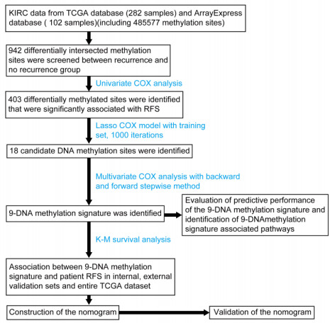
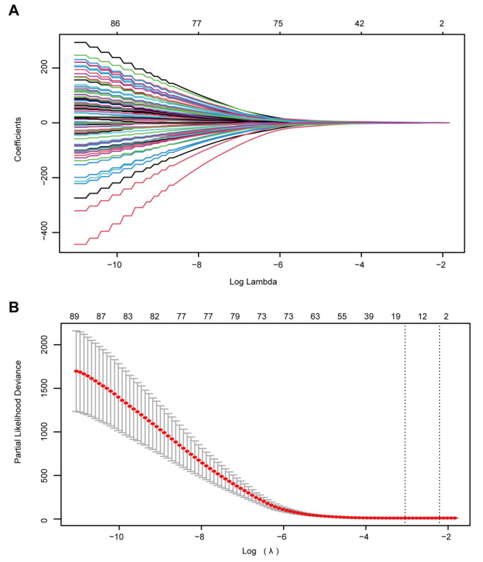
The 282 patients with complete DNA methylation data and corresponding clinical information were selected to construct the prognostic model. The 282 patients were grouped into a training set (70%, n = 198 samples) to determine a prognostic predictor by univariate Cox proportional hazard analysis, least absolute shrinkage and selection operator (LASSO) and multivariate Cox regression analysis. The internal validation set (30%, n = 84) and an external validation set (E-MTAB-3274) were used to validate the predictive value of the predictor by receiver operating characteristic (ROC) analysis and Kaplan–Meier survival analysis.
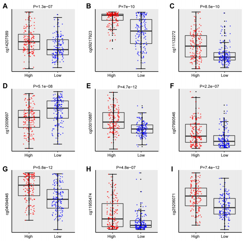
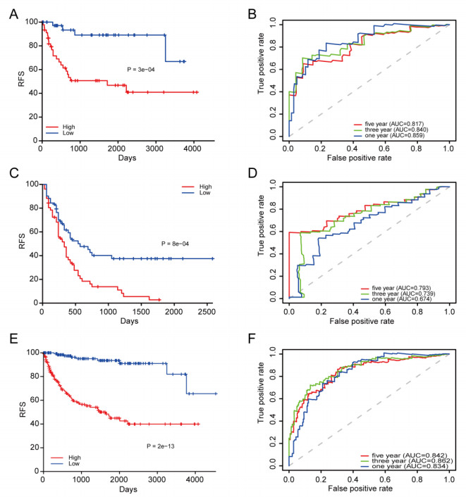
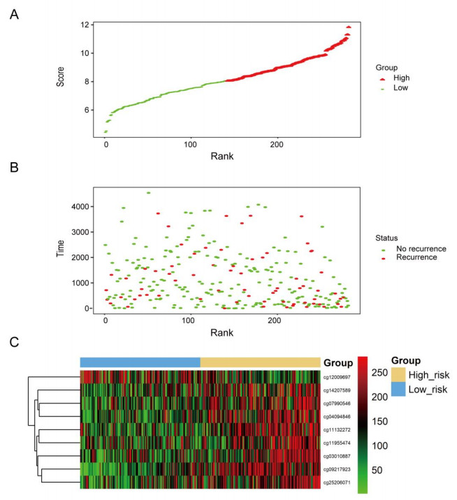
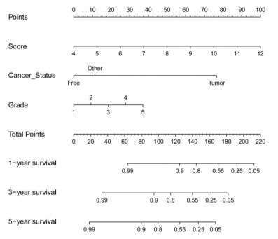
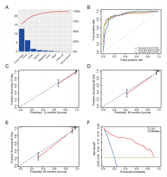
We successfully identified a 9-DNA methylation signature for recurrence free survival (RFS) of KIRC patients. We proved the strong robustness of the 9-DNA methylation signature for predicting RFS through ROC analysis (AUC at 1, 3, 5 years in internal dataset (0.859, 0.840, 0.817, respectively), external validation dataset (0.674, 0.739, 0.793, respectively), entire TCGA dataset (0.834, 0.862, 0.842, respectively)). In addition, a nomogram combining methylation risk score with the conventional clinic-related covariates was constructed to improve the prognostic predicted ability for KIRC patients. The result implied a good performance of the nomogram.
we successfully identified a DNA methylation-associated nomogram, which was helpful in improving the prognostic predictive ability of KIRC patients.
Citation: Xiuxian Zhu, Xianxiong Ma, Chuanqing Wu. A methylomics-correlated nomogram predicts the recurrence free survival risk of kidney renal clear cell carcinoma[J]. Mathematical Biosciences and Engineering, 2021, 18(6): 8559-8576. doi: 10.3934/mbe.2021424
Various studies have suggested that the DNA methylation signatures were promising to identify novel hallmarks for predicting prognosis of cancer. However, few studies have explored the capacity of DNA methylation for prognostic prediction in patients with kidney renal clear cell carcinoma (KIRC). It's very promising to develop a methylomics-related signature for predicting prognosis of KIRC.
The 282 patients with complete DNA methylation data and corresponding clinical information were selected to construct the prognostic model. The 282 patients were grouped into a training set (70%, n = 198 samples) to determine a prognostic predictor by univariate Cox proportional hazard analysis, least absolute shrinkage and selection operator (LASSO) and multivariate Cox regression analysis. The internal validation set (30%, n = 84) and an external validation set (E-MTAB-3274) were used to validate the predictive value of the predictor by receiver operating characteristic (ROC) analysis and Kaplan–Meier survival analysis.
We successfully identified a 9-DNA methylation signature for recurrence free survival (RFS) of KIRC patients. We proved the strong robustness of the 9-DNA methylation signature for predicting RFS through ROC analysis (AUC at 1, 3, 5 years in internal dataset (0.859, 0.840, 0.817, respectively), external validation dataset (0.674, 0.739, 0.793, respectively), entire TCGA dataset (0.834, 0.862, 0.842, respectively)). In addition, a nomogram combining methylation risk score with the conventional clinic-related covariates was constructed to improve the prognostic predicted ability for KIRC patients. The result implied a good performance of the nomogram.
we successfully identified a DNA methylation-associated nomogram, which was helpful in improving the prognostic predictive ability of KIRC patients.

| [1] | R. L. Siegel, K. D. Miller, A. Jemal, Cancer Statistics, CA Cancer J. Clin., 67 (2017), 7-30. |
| [2] | G. Gandaglia, P. Ravi, F. Abdollah, A. E. Abd-El-Barr, A. Becker, I. Popa, et al., Contemporary incidence and mortality rates of kidney cancer in the United States, Can. Urol. Assoc. J., 8 (2014), 247-252. |
| [3] |
D. J. Sanchez, M. C. Simon, Genetic and metabolic hallmarks of clear cell renal cell carcinoma, Biochem. Biophys. Acta Rev. Cancer, 1870 (2018), 23-31. doi: 10.1016/j.bbcan.2018.06.003

|
| [4] | P. Fisel, S. Kruck, S. Winter, J. Bedke, J. Hennenlotter, A. T. Nies, et al., DNA methylation of the SLC16A3 promoter regulates expression of the human lactate transporter MCT4 in renal cancer with consequences for clinical outcome, Clin. Cancer Res., 19 (2013), 5170-5181. |
| [5] | P. Cairns, Renal cell carcinoma, Cancer Biomarks, 9 (2010), 461-473. |
| [6] |
S. H. Rossi, T. Klatte, J. Usher-Smith, G. D. Stewart, Epidemiology and screening for renal cancer, World J. Urol., 36 (2018), 1341-1353. doi: 10.1007/s00345-018-2286-7
|
| [7] | L. Chen, Y. Luo, G. Wang, K. Qian, G. Qian, C. L. Wu, et al., Prognostic value of a gene signature in clear cell renal cell carcinoma, J. Cell Physiol., 234 (2019), 10324-10335. |
| [8] |
L. Guan, J. Tan, H. Li, X. Jin, Biomarker identification in clear cell renal cell carcinoma based on miRNA-seq and digital gene expression-seq data, Gene, 647 (2018), 205-212. doi: 10.1016/j.gene.2017.12.031
|
| [9] | L. Qu, Z. L. Wang, Q. Chen, Y. M. Li, H. W. He, J. J. Hsieh, et al., Prognostic Value of a Long Non-coding RNA Signature in Localized Clear Cell Renal Cell Carcinoma, Eur. Urol., 74 (2018), 756-763. |
| [10] | J. I. Lopez, P. Errarte, A. Erramuzpe, R. Guarch, J. M. Cortes, J. C. Angulo, et al., Fibroblast activation protein predicts prognosis in clear cell renal cell carcinoma, Hum. Pathol., 54 (2016), 100-105. |
| [11] |
N. Ahuja, A. R. Sharma, S. B. Baylin, Epigenetic Therapeutics: A New Weapon in the War Against Cancer, Ann. Rev. Med., 67 (2016), 73-89. doi: 10.1146/annurev-med-111314-035900
|
| [12] |
P. A. Jones, J. P. Issa, S. Baylin, Targeting the cancer epigenome for therapy, Nat. Rev. Genet., 17 (2016), 630-641. doi: 10.1038/nrg.2016.93
|
| [13] | T. W. Grunt, Interacting Cancer Machineries: Cell Signaling, Lipid Metabolism, and Epigenetics, Trends Endocrinol. Metab., 29 (2018), 86-98. |
| [14] | A. Nebbioso, F. P. Tambaro, C. Dell'Aversana, L. Altucci, Cancer epigenetics: Moving forward, PLoS Genet., 14 (2018), e1007362. |
| [15] | M. V. Brock, C. M. Hooker, E. Ota-Machida, Y. Han, M. Guo, S. Ames, et al., DNA methylation markers and early recurrence in stage I lung cancer, N. Eng. J. Med., 358 (2008), 1118-1128. |
| [16] | S. Shen, G. Wang, Q. Shi, R. Zhang, Y. Zhao, Y. Wei, et al., Seven-CpG-based prognostic signature coupled with gene expression predicts survival of oral squamous cell carcinoma, Clin. Epigenet., 9 (2017), 88. |
| [17] | M. Gundert, D. Edelmann, A. Benner, L. Jansen, M. Jia, V. Walter, et al., Genome-wide DNA methylation analysis reveals a prognostic classifier for non-metastatic colorectal cancer (ProMCol classifier), Gut, 68 (2019), 101-110. |
| [18] | D. Capper, D. T. W. Jones, M. Sill, V. Hovestadt, D. Schrimpf, D. Sturm, et al., DNA methylation-based classification of central nervous system tumours, Nature, 555 (2018), 469-474. |
| [19] | A. Colaprico, T. C. Silva, C. Olsen, L. Garofano, C. Cava, D. Garolini, et al., TCGAbiolinks: an R/Bioconductor package for integrative analysis of TCGA data, Nucleic Acids Res., 44 (2016), e71. |
| [20] | I. Merelli, P. Lio, L. Milanesi, NuChart: an R package to study gene spatial neighbourhoods with multi-omics annotations, PLoS One, 8 (2013), e75146. |
| [21] | S. Engebretsen, J. Bohlin, Statistical predictions with glmnet, Clin. Epigenet., 11 (2019), 123. |
| [22] | R. Pidsley, Y. W. CC, M. Volta, K. Lunnon, J. Mill, L. C. Schalkwyk, A data-driven approach to preprocessing Illumina 450K methylation array data, BMC Genom., 14 (2013), 293. |
| [23] | M. J. Aryee, A. E. Jaffe, H. Corrada-Bravo, C. Ladd-Acosta, A. P. Feinberg, K. D. Hansen, et al., Minfi: a flexible and comprehensive Bioconductor package for the analysis of Infinium DNA methylation microarrays, Bioinformatics, 30 (2014), 1363-1369. |
| [24] | X. Robin, N. Turck, A. Hainard, N. Tiberti, F. Lisacek, J. C. Sanchez, et al., pROC: an open-source package for R and S+ to analyze and compare ROC curves, BMC Bioinf., 12 (2011), 77. |
| [25] |
G. De Angelis, R. De Angelis, L. Frova, A. Verdecchia, MIAMOD: a computer package to estimate chronic disease morbidity using mortality and survival data, Comput. Methods Programs Biomed., 44 (1994), 99-107. doi: 10.1016/0169-2607(94)90091-4
|
| [26] | S. Hanzelmann, R. Castelo, J. Guinney, GSVA: gene set variation analysis for microarray and RNA-seq data, BMC Bioinf., 14 (2013), 7. |
| [27] |
X. Liu, J. Wen, C. Li, H. Wang, J. Wang, H. Zou, High-Yield Methylation Markers for Stool-Based Detection of Colorectal Cancer, Dig. Dis. Sci., 65 (2020), 1710-1719. doi: 10.1007/s10620-019-05908-9
|
| [28] |
H. Liao, J. L. Kang, W. Y. Jiang, C. Deng, J. Yuan, R. Shuai, Delivery of Constitutively Active Mutant MKK6(E) With TAT-OSBP Induces Apoptosis in Human Ovarian Carcinoma HO8910 Cells, Int. J. Gynecol. Cancer, 25 (2015), 1548-1556. doi: 10.1097/IGC.0000000000000538
|
| [29] | C. H. Hsing, H. C. Cheng, Y. H. Hsu, C. H. Chan, C. H. Yeh, C. F. Li, et al., Upregulated IL-19 in breast cancer promotes tumor progression and affects clinical outcome, Clin. Cancer Res., 18 (2012), 713-725. |
| [30] |
J. Y. Wang, Y. Zhu, C. F. Wang, S. L. Zhang, B. Dai, D. W. Ye, A nomogram to predict Gleason sum upgrading of clinically diagnosed localized prostate cancer among Chinese patients, Chin. J. Cancer, 33 (2014), 241-248. doi: 10.5732/cjc.013.10137
|
| [31] | C. K. Lee, R. J. Simes, C. Brown, S. Lord, U. Wagner, M. Plante, et al., Prognostic nomogram to predict progression-free survival in patients with platinum-sensitive recurrent ovarian cancer, Br. J. Cancer, 105 (2011), 1144-1150. |
| [32] | S. Taskin, Y. E. Sukur, B. Varli, K. Koyuncu, M. M. Seval, C. Ates, et al., Nomogram with potential clinical use to predict lymph node metastasis in endometrial cancer patients diagnosed incidentally by postoperative pathological assessment, Arch. Gynecol. Obstet., 296 (2017), 803-809. |
| [33] | S. P. Connell, M. Hanna, F. McCarthy, R. Hurst, M. Webb, H. Curley, et al., A Four-Group Urine Risk Classifier for Predicting Outcome in Prostate Cancer Patients, BJU Int., 2019. |
| [34] | Y. Zhang, Z. Li, M. Chen, H. Chen, Q. Zhong, L. Liang, et al., Identification of a New Eight-Long Noncoding RNA Molecular Signature for Breast Cancer Survival Prediction, DNA Cell Biol., 38 (2019), 1529-1539. |
| [35] | Z. Liu, M. Li, Q. Hua, Y. Li, G. Wang, Identification of an eight-lncRNA prognostic model for breast cancer using WGCNA network analysis and a Coxproportional hazards model based on L1-penalized estimation, Int. J. Mol. Med., 44 (2019), 1333-1343. |
| [36] | Q. Du, Y. Wang, S. Guan, C. Hu, M. Li, L. Zhou, et al., The diagnostic nomogram of platelet-based score models for hepatic alveolar echinococcosis and atypical liver cancer, Sci. Rep., 9 (2019), 19403. |
| [37] |
S. M. Kim, Y. Kim, K. Jeong, H. Jeong, J. Kim, Logistic LASSO regression for the diagnosis of breast cancer using clinical demographic data and the BI-RADS lexicon for ultrasonography, Ultrasonography, 37 (2018), 36-42. doi: 10.14366/usg.16045
|
 mbe-18-06-424-Supplementary.pdf mbe-18-06-424-Supplementary.pdf |
 |
Figures(8) / Tables(2)

Xiuxian Zhu, Xianxiong Ma, Chuanqing Wu. A methylomics-correlated nomogram predicts the recurrence free survival risk of kidney renal clear cell carcinoma[J]. Mathematical Biosciences and Engineering, 2021, 18(6): 8559-8576. doi: 10.3934/mbe.2021424


 DownLoad: