Dynamics of drug on-drug off models with mutations in morbidostat — Dedicated to the seventieth birthday of Professor Gail Wolkowicz

Ziran Cheng; Sze-Bi Hsu; Ziran Cheng; Sze-Bi Hsu

doi:10.3934/math.20231061

AIMS Mathematics

2023, Volume 8, Issue 9: 20815-20840. doi: 10.3934/math.20231061

Previous Article Next Article

Research article Special Issues

Dynamics of drug on-drug off models with mutations in morbidostat — Dedicated to the seventieth birthday of Professor Gail Wolkowicz

Ziran Cheng ¹,
Sze-Bi Hsu ^{2
,
,}

1.
Shen Zhen senior high school, Shenzhen, Guan-Dong, China
2.
Department of Mathematics, National Tsing-Hua University, Taiwan

Received: 04 October 2022 Revised: 03 June 2023 Accepted: 20 June 2023 Published: 29 June 2023
MSC : 34C, 92B, 94D

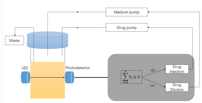
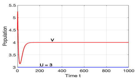
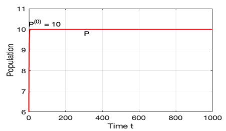
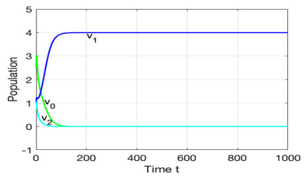
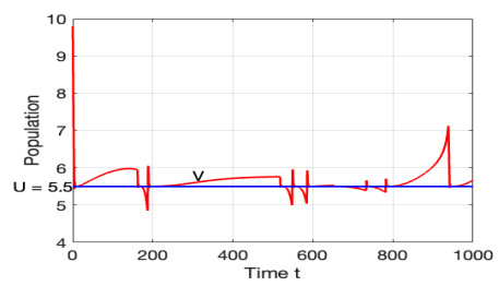
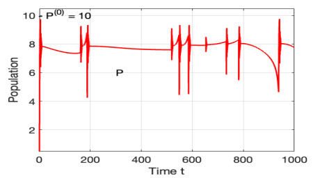
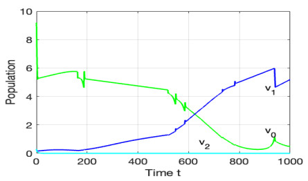
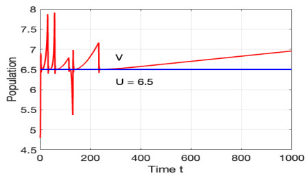
The morbidostat is a bacteria culture device that progressively increases antibiotic drug concentration. It is used to study the evolutionary pathway. In this article, we construct mathematical models for the morbidostat. First we consider the case of no mutations, we study limiting systems and obtain criteria for the large time behavior of the solutions. From the theoretical results and numerical simulations, we conclude that there are two competitive exclusion states of either wild type or mutant type as the threshold parameter $ U $ varies. There are three cases, wild type bacteria excludes all mutants; a mutant dominates in the competition; oscillation between the above two states.

Next we study the systems of forward mutations and forward-backward mutations. Then we apply a result of pertubation for globally stable state.
- morbidostat,
- chemostat,
- wild type,
- mutants,
- drug inhibition,
- exclusion principle,
- coexistence,
- differential inequalities,
- impulse systems
Citation: Ziran Cheng, Sze-Bi Hsu. Dynamics of drug on-drug off models with mutations in morbidostat — Dedicated to the seventieth birthday of Professor Gail Wolkowicz[J]. AIMS Mathematics, 2023, 8(9): 20815-20840. doi: 10.3934/math.20231061

Related Papers:

Abstract

The morbidostat is a bacteria culture device that progressively increases antibiotic drug concentration. It is used to study the evolutionary pathway. In this article, we construct mathematical models for the morbidostat. First we consider the case of no mutations, we study limiting systems and obtain criteria for the large time behavior of the solutions. From the theoretical results and numerical simulations, we conclude that there are two competitive exclusion states of either wild type or mutant type as the threshold parameter $ U $ varies. There are three cases, wild type bacteria excludes all mutants; a mutant dominates in the competition; oscillation between the above two states.

Next we study the systems of forward mutations and forward-backward mutations. Then we apply a result of pertubation for globally stable state.

References

[1]	H. L. Smith, P. E.Waltman, The theory of the chemostat, Cambridge University Press, Cambridge, 1995. https://doi.org/10.1017/CBO9780511530043
[2]	S. B. Hsu, K. C. Chen, Ordinary differential equations with applications, Series on Applied Mathematics, Vol 23, World Scientific Press, 2022, 3rd Edition. https://doi.org/10.1142/8744
[3]	W. A. Coppel, Stability and asymptotic behaivor of differential equations, Health. Math. Monograph, 1965.
[4]	P. Lancaster, M. Tismenetsky, The Theory of Matrices-second edition: With Applications, Academic Press, 1985.
[5]	Z. Chen, S. B. Hsu, Y. T. Yang, The continuous Morbidostat : a chemostat controlled drug application to select for drug resistance mutants, Commun. Pur. Appl. Anal., 19 2020,203–220. https://doi.org/10.3934/cpaa.2020011 doi: 10.3934/cpaa.2020011
[6]	Z. Chen, S. B. Hsu, Y. T. Yang, The Morbidostat: A Bio-reactor That Promotes Selection for Drug Resistance in Bacteria, SIAM J. Appl. Math., 77 (2017), 470–499. https://doi.org/10.1137/16M105695X doi: 10.1137/16M105695X
[7]	H. L. Smith, P. Waltman, Perturbation of a Globally Stable Steady State, Proceedings of the American Mathematical Society, 127 (1999), 447–453. https://doi.org/10.1090/S0002-9939-99-04768-1 doi: 10.1090/S0002-9939-99-04768-1
[8]	M. Barber, Infection by penicillin resistant Staphylococci, Lancet, 2 (1948), 641–644. https://doi.org/10.1016/S0140-6736(48)92166-7 doi: 10.1016/S0140-6736(48)92166-7
[9]	S. B. Levy, B. Marshall, Antibacterial resistance worldwide: causes, challenges and responses, Nat. Med., 10 (2004), s122–s129. https://doi.org/10.1038/nm1145 doi: 10.1038/nm1145
[10]	E. Toprak, A. Veres, S. Yildiz, J. M. Pedraza, R. Chait, J. Paulsson, et al., Building a morbidostat: an automated continuous-culturre device for studying bacterial drug resistance under dynamically sustained drug inhibition, Nat. protoc., 8 (2013), 555–567. https://doi.org/10.1038/nprot.2013.021 doi: 10.1038/nprot.2013.021
[11]	E. Toprak, A. Veres, J. B. Michel, R. Chait, D. L. Hartl, R. Kishony, Evolutionary paths to antibiotic resistance under dynamically sustained drug selection, Nat. Genet., 44 (2012), 101–105.

Reader Comments

Your name:*

Email:*
© 2023 the Author(s), licensee AIMS Press. This is an open access article distributed under the terms of the Creative Commons Attribution License (http://creativecommons.org/licenses/by/4.0)