Current air-conditioning and refrigeration systems utilize active cooling technology, which consumes a lot of energy from fossil fuels, thereby increasing global warming and depletion of the ozone layer. Passive cooling is considered an alternative to active cooling because it is effective and less expensive and does not require the use of electricity, so cooling can be achieved in locations where there is no electricity. Hydrogels are flexible and soft 3-dimensional networks with high water content and evaporative and radiative cooling properties that make them suitable for use in passive cooling technology. Natural hydrogels are considered alternatives to synthetic hydrogels because they are biodegradable, biocompatible, sensitive to external environments and mostly sourced from plant-based sources. There are limited studies on the application of mucilage-based hydrogel for passive cooling, despite its excellent thermal, mechanical and physiochemical properties. Therefore, this study evaluates the properties of mucilage-based hydrogel as a plausible alternative to synthetic hydrogel for passive cooling. The possibility of using mucilage-based hydrogel in passive cooling technology depends on the mucilage biomass feedstock, mucilage extraction techniques, polymerization techniques and additives introduced into the hydrogel matrix. Different mucilage extraction techniques; mucilage percentage yield; the effects of crosslinkers, polymers and nanoparticle additives on the properties of mucilage-based hydrogel; and the potential of using mucilage-based hydrogel for passive cooling technology are examined in this review.
Citation: Mercy Ogbonnaya, Abimbola P.I Popoola. Potential of mucilage-based hydrogel for passive cooling technology: Mucilage extraction techniques and elucidation of thermal, mechanical and physiochemical properties of mucilage-based hydrogel[J]. AIMS Materials Science, 2023, 10(6): 1045-1076. doi: 10.3934/matersci.2023056
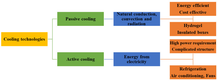
Current air-conditioning and refrigeration systems utilize active cooling technology, which consumes a lot of energy from fossil fuels, thereby increasing global warming and depletion of the ozone layer. Passive cooling is considered an alternative to active cooling because it is effective and less expensive and does not require the use of electricity, so cooling can be achieved in locations where there is no electricity. Hydrogels are flexible and soft 3-dimensional networks with high water content and evaporative and radiative cooling properties that make them suitable for use in passive cooling technology. Natural hydrogels are considered alternatives to synthetic hydrogels because they are biodegradable, biocompatible, sensitive to external environments and mostly sourced from plant-based sources. There are limited studies on the application of mucilage-based hydrogel for passive cooling, despite its excellent thermal, mechanical and physiochemical properties. Therefore, this study evaluates the properties of mucilage-based hydrogel as a plausible alternative to synthetic hydrogel for passive cooling. The possibility of using mucilage-based hydrogel in passive cooling technology depends on the mucilage biomass feedstock, mucilage extraction techniques, polymerization techniques and additives introduced into the hydrogel matrix. Different mucilage extraction techniques; mucilage percentage yield; the effects of crosslinkers, polymers and nanoparticle additives on the properties of mucilage-based hydrogel; and the potential of using mucilage-based hydrogel for passive cooling technology are examined in this review.

| [1] |
Lickley M, Solomon S, Fletcher S, et al. (2020) Quantifying contributions of chlorofluorocarbon banks to emissions and impacts on the ozone layer and climate. Nat Commun 11: 1380. https://doi.org/10.1038/s41467-020-15162-7 doi: 10.1038/s41467-020-15162-7

|
| [2] |
Madduma-Bandarage USK, Madihally SV (2021) Synthetic hydrogels: Synthesis, novel trends, and applications. J Appl Polym Sci 138: e50376. https://doi.org/10.1002/app.50376 doi: 10.1002/app.50376
|
| [3] |
Zhao W, Jin X, Cong Y, et al. (2013) Degradable natural polymer hydrogels for articular cartilage tissue engineering. J Chem Technol Biotechnol 88: 327–339. https://doi.org/10.1002/jctb.3970 doi: 10.1002/jctb.3970
|
| [4] |
Rehman WU, Asim M, Hussain S, et al. (2020) Hydrogel: A promising material in pharmaceutics. Curr Pharm Des 26: 5892–5908. https://doi.org/10.2174/1381612826666201118095523 doi: 10.2174/1381612826666201118095523
|
| [5] |
Rajendran JV, Thomas S, Jafari Z, et al. (2022) Recent advances on large-scale manufacture of curcumin and its nanoformulation for cancer therapeutic application. Biointerface Res Appl Chem 12: 7863–7885. https://doi.org/10.33263/BRIAC126.78637885 doi: 10.33263/BRIAC126.78637885
|
| [6] |
Loo HL, Goh BH, Lee LH, et al. (2022) Application of chitosan-based nanoparticles in skin wound healing. Asian J Pharm Sci 17: 299–332. https://doi.org/10.1016/j.ajps.2022.04.001 doi: 10.1016/j.ajps.2022.04.001
|
| [7] |
Liu RR, Shi QQ, Meng YF, et al. (2023) Biomimetic chitin hydrogel via chemical transformation. Nano Res 4: 1–7. https://doi.org/10.1007/s12274-023-5886-5 doi: 10.1007/s12274-023-5886-5
|
| [8] |
Michelini L, Probo L, Farè S, et al. (2020) Characterization of gelatin hydrogels derived from different animal sources. Mater Lett 272: 127865. https://doi.org/10.1016/j.matlet.2020.127865 doi: 10.1016/j.matlet.2020.127865
|
| [9] |
Tosif MM, Najda A, Bains A, et al. (2021) A comprehensive review on plant-derived mucilage: Characterization, functional properties, applications, and its utilization for nanocarrier fabrication. Polymers 13: 1066. https://doi.org/10.3390/polym13071066 doi: 10.3390/polym13071066
|
| [10] |
Cakmak H, Ilyasoglu-Buyukkestelli H, Sogut E, et al. (2023) A review on recent advances of plant mucilages and their applications in food industry: Extraction, functional properties and health benefits. Food Hydrocolloids Health 3: 100131. https://doi.org/10.1016/j.fhfh.2023.100131 doi: 10.1016/j.fhfh.2023.100131
|
| [11] |
Beikzadeh S, Khezerlou A, Jafari SM, et al. (2020) Seed mucilages as the functional ingredients for biodegradable films and edible coatings in the food industry. Adv Colloid Interfac 280: 102164. https://doi.org/10.1016/j.cis.2020.102164 doi: 10.1016/j.cis.2020.102164
|
| [12] |
Chiang JH, Ong DSM, Ng FSK, et al. (2021) Application of chia (Salvia hispanica) mucilage as an ingredient replacer in foods. Trends Food Sci Tech 115: 105–116. https://doi.org/10.1016/j.tifs.2021.06.039 doi: 10.1016/j.tifs.2021.06.039
|
| [13] |
Timilsena YP, Adhikari R, Kasapis S, et al. (2016) Molecular and functional characteristics of purified gum from Australian chia seeds. Carbohyd Polym 136: 128–136. https://doi.org/10.1016/j.carbpol.2015.09.035 doi: 10.1016/j.carbpol.2015.09.035
|
| [14] |
Rostamabadi MM, Falsafi SR, Nishinari K, et al. (2023) Seed gum-based delivery systems and their application in encapsulation of bioactive molecules. Crit Rev Food Sci 63: 9937–9960. https://doi.org/10.1080/10408398.2022.2076065 doi: 10.1080/10408398.2022.2076065
|
| [15] |
Hesarinejad MA, Sami Jokandan M, Mohammadifar MA, et al. (2018) The effects of concentration and heating-cooling rate on rheological properties of Plantago lanceolata seed mucilage. Int J Biol Macromol 115: 1260–1266. https://doi.org/10.1016/j.ijbiomac.2017.10.102 doi: 10.1016/j.ijbiomac.2017.10.102
|
| [16] |
Olawuyi IF, Kim SR, Lee WY (2021) Application of plant mucilage polysaccharides and their techno-functional properties' modification for fresh produce preservation. Carbohyd Polym 272: 118371. https://doi.org/10.1016/j.carbpol.2021.118371 doi: 10.1016/j.carbpol.2021.118371
|
| [17] |
Sacco P, Lipari S, Cok M, et al. (2021) Insights into mechanical behavior and biological properties of chia seed mucilage hydrogels. Gels 7: 47. https://doi.org/10.3390/gels7020047 doi: 10.3390/gels7020047
|
| [18] |
Liu Y, Liu Z, Zhu X, et al. (2021) Seed coat mucilages: Structural, functional/bioactive properties, and genetic information. Compr Rev Food Sci Food Saf 20: 11–26. https://doi.org/10.1111/1541-4337.12742 doi: 10.1111/1541-4337.12742
|
| [19] |
Halász K, Tóth A, Börcsök Z, et al. (2022) Edible antioxidant films from ultrasonically extracted Plantago psyllium seed husk flour mucilage. J Polym Environ 30: 2685–2694. https://doi.org/10.1007/s10924-022-02409-1 doi: 10.1007/s10924-022-02409-1
|
| [20] |
Safdar B, Zhihua P, Xinqi L, et al. (2020) Influence of different extraction techniques on recovery, purity, antioxidant activities, and microstructure of flaxseed gum. J Food Sci 85: 3168–3182. https://doi.org/10.1111/1750-3841.15426 doi: 10.1111/1750-3841.15426
|
| [21] |
Niknam R, Ghanbarzadeh B, Ayaseh A, et al. (2020) Barhang (Plantago major L.) seed gum: Ultrasound-assisted extraction optimization, characterization, and biological activities. J Food Process Preserv 44: e14750. https://doi.org/10.1111/jfpp.14750 doi: 10.1111/jfpp.14750
|
| [22] |
Dybka-Stępień K, Otlewska A, Góźdź P, et al. (2021) The renaissance of plant mucilage in health promotion and industrial applications: A review. Nutrients 13: 3354. https://doi.org/10.3390/nu13103354 doi: 10.3390/nu13103354
|
| [23] |
Ang AMG, Raman IC (2019) Characterization of mucilages from abelmoschus manihot linn., amaranthus spinosus linn. and talinum triangulare (jacq.) willd. leaves for pharmaceutical excipient application. Asian J Biol Life Sci 8: 16–24. https://doi.org/10.5530/ajbls.2019.8.3 doi: 10.5530/ajbls.2019.8.3
|
| [24] |
Ma F, Wang R, Li X, et al. (2020) Physical properties of mucilage polysaccharides from Dioscorea opposita Thunb. Food Chem 311: 126039. https://doi.org/10.1016/j.foodchem.2019.126039 doi: 10.1016/j.foodchem.2019.126039
|
| [25] |
Nazir S, Wani IA, Masoodi FA (2017) Extraction optimization of mucilage from Basil (Ocimum basilicum L.) seeds using response surface methodology. J Adv Res 8: 235–244. https://doi.org/10.1016/j.jare.2017.01.003 doi: 10.1016/j.jare.2017.01.003
|
| [26] |
Tosif MM, Najda A, Klepacka J, et al. (2022) Concise review on taro mucilage: Extraction techniques, chemical composition, characterization, applications, and health attributes. Polymers 14: 1163. https://doi.org/10.3390/polym14061163 doi: 10.3390/polym14061163
|
| [27] |
Estévez AM, Saenz C, Hurtado ML, et al. (2004) Extraction methods and some physical properties of mesquite (Prosopis chilensis (Mol) Stuntz) seed gum. J Sci Food Agric 84: 1487–1492. https://doi.org/10.1002/jsfa.1795 doi: 10.1002/jsfa.1795
|
| [28] |
Quintero-García M, Gutiérrez-Cortez E, Bah M, et al. (2021) Comparative analysis of the chemical composition and physicochemical properties of the mucilage extracted from fresh and dehydrated opuntia ficus indica cladodes. Foods 10: 2137. https://doi.org/10.3390/foods10092137 doi: 10.3390/foods10092137
|
| [29] |
Rodríguez-González S, Martínez-Flores HE, Chávez-Moreno CK, et al. (2014) Extraction and characterization of mucilage from wild species of opuntia. J Food Process Eng 37: 285–292. https://doi.org/10.1111/jfpe.12084 doi: 10.1111/jfpe.12084
|
| [30] |
Kassem IAA, Joshua Ashaolu T, Kamel R, et al. (2021) Mucilage as a functional food hydrocolloid: Ongoing and potential applications in prebiotics and nutraceuticals. Food Funct 12: 4738–4748. https://doi.org/10.1039/d1fo00438g doi: 10.1039/d1fo00438g
|
| [31] |
Waghmare R, Preethi R, Moses JA, et al. (2022) Mucilages: Sources, extraction methods, and characteristics for their use as encapsulation agents. Crit Rev Food Sci Nutr 62: 4186–4207. https://doi.org/10.1080/10408398.2021.1873730 doi: 10.1080/10408398.2021.1873730
|
| [32] |
Capello C, Fischer U, Hungerbuhler K (2007) What is a green solvent? A comprehensive framework for the environmental assessment of solvents. Green Chem 9: 927–934. https://doi.org/10.1039/b617536h doi: 10.1039/b617536h
|
| [33] |
Tian S, Hao C, Xu G, et al. (2017) Optimization conditions for extracting polysaccharide from Angelica sinensis and its antioxidant activities. J Food and Drug Anal 25: 766–775. https://doi.org/10.1016/j.jfda.2016.08.012 doi: 10.1016/j.jfda.2016.08.012
|
| [34] |
Cong Q, Chen H, Liao W, et al. (2016) Structural characterization, and effect on anti-angiogenic activity of a fucoidan from Sargassum fusiforme. Carbohyd Polym 136: 899–907. https://doi.org/10.1016/j.carbpol.2015.09.087 doi: 10.1016/j.carbpol.2015.09.087
|
| [35] |
Saifullah Md, McCullum R, Vuong QV (2021) Optimization of microwave–assisted extraction of polyphenols from lemon myrtle: Comparison of modern and conventional extraction techniques based on bioactivity and total polyphenols in dry extracts. Processes 9: 2212. https://doi.org/10.3390/pr9122212 doi: 10.3390/pr9122212
|
| [36] |
Desai M, Parikh J, Parikh PA (2010) Extraction of natural products using microwaves as a heat source. Sep Purif Rev 39: 1–32. https://doi.org/10.1080/15422111003662320 doi: 10.1080/15422111003662320
|
| [37] |
Chen C, Zhang B, Huang Q, et al. (2017) Microwave-assisted extraction of polysaccharides from Moringa oleifera Lam. leaves: Characterization and hypoglycemic activity. Ind Crop Prod 100: 1–11. https://doi.org/10.1016/j.indcrop.2017.01.042 doi: 10.1016/j.indcrop.2017.01.042
|
| [38] |
Shiehnezhad M, Zarringhalami S, Malekjani N (2023) Optimization of microwave-assisted extraction of mucilage from ocimum basilicum var. album (l.) seed. J Food Process 2023: 552462. https://doi.org/10.1155/2023/5524621 doi: 10.1155/2023/5524621
|
| [39] |
Al-Dhabi NA, Ponmurugan K (2020) Microwave assisted extraction and characterization of polysaccharide from waste jamun fruit seeds. Int J Biol Macromol 152: 1157–1163. https://doi.org/10.1016/j.ijbiomac.2019.10.204 doi: 10.1016/j.ijbiomac.2019.10.204
|
| [40] |
Han YL, Gao J, Yin YY, et al. (2016) Extraction optimization by response surface methodology of mucilage polysaccharide from the peel of Opuntia dillenii haw. fruits and their physicochemical properties. Carbohyd Polym 151: 381–391. https://doi.org/10.1016/j.carbpol.2016.05.085 doi: 10.1016/j.carbpol.2016.05.085
|
| [41] |
Felkai-Haddache L, Dahmoune F, Remini H, et al. (2016) Microwave optimization of mucilage extraction from Opuntia ficus indica Cladodes. Int J Biol Macromol 84: 24–30. https://doi.org/10.1016/j.ijbiomac.2015.11.090 doi: 10.1016/j.ijbiomac.2015.11.090
|
| [42] |
Zhao JL, Zhang M, Zhou HL (2019) Microwave-assisted extraction, purification, partial characterization, and bioactivity of polysaccharides from panax ginseng. Molecules 24: 1605. https://doi.org/10.3390/molecules24081605 doi: 10.3390/molecules24081605
|
| [43] |
Wei E, Yang R, Zhao H, et al. (2019) Microwave-assisted extraction releases the antioxidant polysaccharides from seabuckthorn (Hippophae rhamnoides L.) berries. Int J Biol Macromol 123: 280–290. https://doi.org/10.1016/j.ijbiomac.2018.11.074 doi: 10.1016/j.ijbiomac.2018.11.074
|
| [44] |
Castejón N, Luna P, Señoráns FJ (2017) Ultrasonic removal of mucilage for pressurized liquid extraction of omega-3 rich oil from chia seeds (Salvia hispanica L.). J Agric Food Chem 65: 2572–2579. https://doi.org/10.1021/acs.jafc.6b05726 doi: 10.1021/acs.jafc.6b05726
|
| [45] |
Huang S, Ning Z (2010) Extraction of polysaccharide from Ganoderma lucidum and its immune enhancement activity. Int J Biol Macromol 47: 336–341. https://doi.org/10.1016/j.ijbiomac.2010.03.019 doi: 10.1016/j.ijbiomac.2010.03.019
|
| [46] |
Hedayati S, Niakousari M, Babajafari S, et al. (2021) Ultrasound-assisted extraction of mucilaginous seed hydrocolloids: Physicochemical properties and food applications. Trends Food Sci Tech 118: 356–361. https://doi.org/10.1016/j.tifs.2021.10.022 doi: 10.1016/j.tifs.2021.10.022
|
| [47] |
Wang W, Ma X, Xu Y, et al. (2015) Ultrasound-assisted heating extraction of pectin from grapefruit peel: Optimization and comparison with the conventional method. Food Chem 178: 106–114. https://doi.org/10.1016/j.foodchem.2015.01.080 doi: 10.1016/j.foodchem.2015.01.080
|
| [48] |
Majzoobi M, Hedayati S, Farahnaky A (2015) Functional properties of microporous wheat starch produced by α-amylase and sonication. Food Biosci 11: 79–84. https://doi.org/10.1016/j.fbio.2015.05.001 doi: 10.1016/j.fbio.2015.05.001
|
| [49] |
Pereira GA, Silva EK, Peixoto Araujo NM, et al. (2019) Obtaining a novel mucilage from mutamba seeds exploring different high-intensity ultrasound process conditions. Ultrasonics Sonochem 55: 332–340. https://doi.org/10.1016/j.ultsonch.2019.01.010 doi: 10.1016/j.ultsonch.2019.01.010
|
| [50] |
Zhao X, Qiao L, Wu AM (2017) Effective extraction of Arabidopsis adherent seed mucilage by ultrasonic treatment. Sci Rep 7: 40672. https://doi.org/10.1038/srep40672 doi: 10.1038/srep40672
|
| [51] |
Akhtar MN, Mushtaq Z, Ahmad N, et al. (2019) Optimal ultrasound-assisted process extraction, characterization, and functional product development from flaxseed meal derived polysaccharide gum. Processes 7: 189. https://doi.org/10.3390/pr7040189 doi: 10.3390/pr7040189
|
| [52] |
Souza GS, de Cassia Bergamasco R, Stafussa AP, et al. (2020) Ultrasound-assisted extraction of Psyllium mucilage: Evaluation of functional and technological properties. Emir J Food Agr 32: 238–244. https://doi.org/10.9755/ejfa.2020.v32.i4.2089 doi: 10.9755/ejfa.2020.v32.i4.2089
|
| [53] |
Silva LA, Sinnecker P, Cavalari AA, et al. (2022) Extraction of chia seed mucilage: Effect of ultrasound application. Food Chem Adv 1: 100024. https://doi.org/10.1016/j.focha.2022.100024 doi: 10.1016/j.focha.2022.100024
|
| [54] |
Zhu C, Zhai X, Li L, et al. (2015) Response surface optimization of ultrasound-assisted polysaccharides extraction from pomegranate peel. Food Chem 177: 139–146. https://doi.org/10.1016/j.foodchem.2015.01.022 doi: 10.1016/j.foodchem.2015.01.022
|
| [55] |
Yeh YC, Lai LS (2022) Effect of extraction procedures with ultrasound and cellulolytic enzymes on the structural and functional properties of Citrus grandis Osbeck seed mucilage. Molecules 27: 612. https://doi.org/10.3390/molecules27030612 doi: 10.3390/molecules27030612
|
| [56] |
Kim JH, Lee HJ, Park Y, et al. (2013) Mucilage removal from cactus cladodes (Opuntia humifusa Raf.) by enzymatic treatment to improve extraction efficiency and radical scavenging activity. Lwt-Food Sci Technol 51: 337–342. https://doi.org/10.1016/j.lwt.2012.10.009 doi: 10.1016/j.lwt.2012.10.009
|
| [57] |
Chiang CF, Lai LS (2019) Effect of enzyme-assisted extraction on the physicochemical properties of mucilage from the fronds of Asplenium australasicum (J. Sm.) Hook. Int J Biol Macromol 124: 346–353. https://doi.org/10.1016/j.ijbiomac.2018.11.181 doi: 10.1016/j.ijbiomac.2018.11.181
|
| [58] |
Zeng W, Lai L (2016) Characterization of the mucilage extracted from the edible fronds of bird's nest fern (Asplenium australasicum) with enzymatic modifications. Food Hydrocolloid 53: 84–92. https://doi.org/10.1016/j.foodhyd.2015.03.02 doi: 10.1016/j.foodhyd.2015.03.02
|
| [59] |
Tavares LS, Junqueira LA, Guimarães ICO, et al. (2018) Cold extraction method of chia seed mucilage (Salvia hispanica L.): Effect on yield and rheological behavior. J Food Sci Technol 55: 457–466. https://doi.org/10.1007/s13197-017-2954-4 doi: 10.1007/s13197-017-2954-4
|
| [60] |
Mutlu S, Kopuk B, Palabiyik I (2023) Effect of cold atmospheric pressure argon plasma jet treatment on the freeze-dried mucilage of chia seeds (salvia hispanica l.). Foods 12: 1563. https://doi.org/10.3390/foods12081563 doi: 10.3390/foods12081563
|
| [61] |
Li X, Zhang ZH, Qi X, et al. (2021) Application of nonthermal processing technologies in extracting and modifying polysaccharides: A critical review. Compr Rev Food Sci Food Saf 20: 4367–4389. https://doi.org/10.1111/1541-4337.12820 doi: 10.1111/1541-4337.12820
|
| [62] |
Ramazzina I, Berardinelli A, Rizzi F, et al. (2015) Effect of cold plasma treatment on physicochemical parameters and antioxidant activity of minimally processed kiwifruit. Postharvest Biol Technol 107: 55–65. https://doi.org/10.1016/j.postharvbio.2015.04.008 doi: 10.1016/j.postharvbio.2015.04.008
|
| [63] |
Mehta D, Purohit A, Bajarh P, et al. (2022) Cold plasma processing improved the extraction of xylooligosaccharides from dietary fibers of rice and corn bran with enhanced in-vitro digestibility and anti-inflammatory responses. Innov Food Sci Emerg Technol 78: 103027. https://doi.org/10.1016/j.ifset.2022.103027 doi: 10.1016/j.ifset.2022.103027
|
| [64] |
Brasoveanu M, Nemtanu MR (2020) Pasting properties modelling and comparative analysis of starch exposed to ionizing radiation. Radiat Phys Chem 168: 108492. https://doi.org/10.1016/j.radphyschem.2019:108492 doi: 10.1016/j.radphyschem.2019.108492
|
| [65] |
Zielinska S, Cybulska J, Pieczywek P, et al. (2022) Structural morphology and rheological properties of pectin fractions extracted from okra pods subjected to cold plasma treatment. Food Bioprocess Technol 15: 1168–1181. https://doi.org/10.1007/s11947-022-02798-0 doi: 10.1007/s11947-022-02798-0
|
| [66] |
Muñoz LA, Cobos A, Diaz O, et al. (2012) Chia seeds: Microstructure, mucilage extraction and hydration. J Food Eng 108: 216–224. https://doi.org/10.1016/j.jfoodeng.2011.06.037 doi: 10.1016/j.jfoodeng.2011.06.037
|
| [67] |
Wang WH, Lu CP, Kuo MI (2022) Combination of ultrasound and heat in the extraction of chia seed (salvia hispanica l.) mucilage: Impact on yield and technological properties. Processes 10: 519. https://doi.org/10.3390/pr10030519 doi: 10.3390/pr10030519
|
| [68] |
Xue X, Hu Y, Wang S, et al. (2022) Fabrication of physical and chemical crosslinked hydrogels for bone tissue engineering. Bioact Mater 12: 327–339. https://doi.org/10.1016/j.bioactmat.2021.10.029 doi: 10.1016/j.bioactmat.2021.10.029
|
| [69] |
Hu W, Wang Z, Xiao Y, et al. (2019) Advances in crosslinking strategies of biomedical hydrogels. Biomater Sci 7: 843–855. https://doi.org/10.1039/C8BM01246F doi: 10.1039/C8BM01246F
|
| [70] |
Parhi R (2017) Cross-linked hydrogel for pharmaceutical applications: A review. Adv Pharm Bull 7: 515–530. https://doi.org/10.15171/apb.2017.064 doi: 10.15171/apb.2017.064
|
| [71] | Palencia M, Lerma TA, Garcés V, et al. (2021) Eco-friendly hydrogels, In: Palencia M, Lerma TA, Garcés V, et al. Eco-friendly Functional Polymers, Amsterdam: Elsevier, 141–153. https://doi.org/10.1016/B978-0-12-821842-6.00015-4 |
| [72] |
Samateh M, Pottackal N, Manafirasi S, et al. (2018) Unravelling the secret of seed-based gels in water: The nanoscale 3D network formation. Sci Rep 8: 7315. https://doi.org/10.1038/s41598-018-25691-3 doi: 10.1038/s41598-018-25691-3
|
| [73] |
Sharma G, Kumar A, Devi K, et al. (2018) Guar gum-crosslinked-Soya lecithin nanohydrogel sheets as effective adsorbent for the removal of thiophanate methyl fungicide. Int J Biol Macromol 114: 295–305. https://doi.org/10.1016/j.ijbiomac.2018.03.093 doi: 10.1016/j.ijbiomac.2018.03.093
|
| [74] |
Deore UV, Mahajan HS (2022) Hydrogel for topical drug delivery based on Mimosa pudica seed mucilage: Development and characterization. Sustain Chem Pharm 27: 100701. https://doi.org/10.1016/j.scp.2022.100701 doi: 10.1016/j.scp.2022.100701
|
| [75] |
Sharma R, Gupta RK, Rani A (2023) Hydrogels based on mucilage of underutilized cereals: Synthesis and characterization. Indian J Chem Techn 30: 524–533. https://doi.org/10.56042/ijct.v30i4.70238 doi: 10.56042/ijct.v30i4.70238
|
| [76] |
Mahmood A, Erum A, Mumtaz S, et al. (2022) Preliminary investigation of linum usitatissimum mucilage-based hydrogel as possible substitute to synthetic polymer-based hydrogels for sustained release oral drug delivery. Gels 8: 170. https://doi.org/10.3390/gels8030170 doi: 10.3390/gels8030170
|
| [77] | Choudhary V, Sharma S, Shukla PK, et al. (2023) Biocompatible stimuli responsive hydrogels of okra mucilage with acrylic acid for controlled release phytochemicals of Calendula officinalis: In vitro assay. Mater Today Proc (in press). https://doi.org/10.1016/j.matpr.2023.03.701 |
| [78] |
Rodríguez-Loredo NA, Ovando-Medina VM, Pérez E, et al. (2023) Preparation of poly(acrylic acid)/linseed mucilage/chitosan hydrogel for ketorolac release. J Vinyl Addit Technol 29: 890–900. https://doi.org/10.1002/vnl.22023 doi: 10.1002/vnl.22023
|
| [79] |
Hosseini MS, Hemmati K, Ghaemy M (2016) Synthesis of nanohydrogels based on tragacanth gum biopolymer and investigation of swelling and drug delivery. Int J Biol Macromol 82: 806–815. https://doi.org/10.1016/j.ijbiomac.2015.09.067 doi: 10.1016/j.ijbiomac.2015.09.067
|
| [80] |
Moya-Ortega MD, Alvarez-Lorenzo C, Sigurdsson HH, et al. (2012) Cross-linked hydroxypropyl-β-cyclodextrin and γ-cyclodextrin nanogels for drug delivery: Physicochemical and loading/release properties. Carbohyd Polym 87: 2344–2351. https://doi.org/10.1016/j.carbpol.2011.11.005 doi: 10.1016/j.carbpol.2011.11.005
|
| [81] |
Pathania D, Verma C, Negi P, et al. (2018) Novel nanohydrogel based on itaconic acid grafted tragacanth gum for controlled release of ampicillin. Carbohyd Polym 196: 262–271. https://doi.org/10.1016/j.carbpol.2018.05.040 doi: 10.1016/j.carbpol.2018.05.040
|
| [82] |
Dalwadi C, Patel G (2015) Application of nanohydrogels in drug delivery systems: Recent patents review. Recent Pat Nanotechnol 9: 17–25. https://doi.org/10.2174/1872210509666150101151521 doi: 10.2174/1872210509666150101151521
|
| [83] |
Sabzevar SM, Mehrshad ZM, Naimipour M (2021) A biological magnetic nano-hydrogel based on basil seed mucilage: Study of swelling ratio and drug delivery. Iran Polym J 30: 485–493. https://doi.org/10.1007/s13726-021-00905-0 doi: 10.1007/s13726-021-00905-0
|
| [84] |
Archana, Suman A, Singh V (2022) An inclusive review on mucilage: Extraction methods, characterization, and its utilization for nanocarriers manufacturing. J Drug Delivery Ther 12: 171–179. https://doi.org/10.22270/jddt.v12i1-S.5210 doi: 10.22270/jddt.v12i1-S.5210
|
| [85] |
Sen S, Bal T, Rajora AD (2022) Green nanofiber mat from HLM–PVA–Pectin (Hibiscus leaves mucilage–polyvinyl alcohol–pectin) polymeric blend using electrospinning technique as a novel material in wound-healing process. Appl Nanosci 12: 237–250. https://doi.org/10.1007/s13204-021-02295-4 doi: 10.1007/s13204-021-02295-4
|
| [86] |
Emadzadeh MK, Aarabi A, Aarabi Najvani F, et al. (2022) The effect of extraction method on physicochemical properties of mucilage extracted from yellow and brown flaxseeds. Jundishapur J Nat Pharm Prod 17: e123952. https://doi.org/10.5812/jjnpp-123952 doi: 10.5812/jjnpp-123952
|
| [87] |
Wang X, Wu Y, Chen G, et al. (2013) Optimisation of ultrasound assisted extraction of phenolic compounds from Sparganii rhizoma with response surface methodology. Ultrason Sonochem 20: 846–854. https://doi.org/10.1016/j.ultsonch.2012.11.007 doi: 10.1016/j.ultsonch.2012.11.007
|
| [88] |
Guo Y, Bae J, Fang Z, et al. (2020) Hydrogels and hydrogel-derived materials for energy and water sustainability. Chem Rev 120: 7642–7707. https://doi.org/10.1021/acs.chemrev.0c00345 doi: 10.1021/acs.chemrev.0c00345
|
| [89] |
Chai Q, Jiao Y, Yu X (2017) Hydrogels for biomedical applications: Their characteristics and the mechanisms behind them. Gels 3: 6. https://doi.org/10.3390/gels3010006 doi: 10.3390/gels3010006
|
| [90] | Ganji F, Vasheghani FS, Vasheghani FE (2010) Theoretical description of hydrogel swelling: A review. Iran Polym J 19: 375–398. |
| [91] |
Nerkar PP, Gattani S (2011) In vivo, in vitro evaluation of linseed mucilage based buccal mucoadhesive microspheres of venlafaxine. Drug Deliv 18: 111–121. https://doi.org/10.3109/10717544.2010.520351 doi: 10.3109/10717544.2010.520351
|
| [92] |
Sumaira, Ume RT, Alia E, et al. (2021) Fabrication, characterization, and toxicity evaluation of chemically cross-linked polymeric network for sustained delivery of metoprolol tartrate. Des Monomers Polym 24: 351–361. https://doi.org/10.1080/15685551.2021.2003995 doi: 10.1080/15685551.2021.2003995
|
| [93] |
Xu L, Sun DW, Tian Y, et al. (2022) Combined effects of radiative and evaporative cooling on fruit preservation under solar radiation: Sunburn resistance and temperature stabilization. ACS Appl Mater Interfaces 14: 45788–45799. https://doi.org/10.1021/acsami.2c11349 doi: 10.1021/acsami.2c11349
|
| [94] |
Ninan N, Muthiah M, Park IK, et al. (2013) Pectin/carboxymethyl cellulose/microfibrillated cellulose composite scaffolds for tissue engineering. Carbohyd Polym 98: 877–885. https://doi.org/10.1016/j.carbpol.2013.06.067 doi: 10.1016/j.carbpol.2013.06.067
|
| [95] |
Zhou Z, Qian C, Yuan W (2021) Self-healing, anti-freezing, adhesive and remoldable hydrogel sensor with ion-liquid metal dual conductivity for biomimetic skin. Compos Sci Technol 203: 108608. https://doi.org/10.1016/j.compscitech.2020.108608 doi: 10.1016/j.compscitech.2020.108608
|
| [96] |
Quinzio CM, Ayunta CA, Alancay MM, et al. (2018) Physicochemical and rheological properties of mucilage extracted from Opuntia ficus indica (L. Miller). Comparative study with guar gum and xanthan gum. Food Measure 12: 459–470. https://doi.org/10.1007/s11694-017-9659-2 doi: 10.1007/s11694-017-9659-2
|
| [97] |
Martin AA, de Freitas RA, Sassaki GL, et al. (2017) Chemical structure and physical-chemical properties of mucilage from the leaves of Pereskia aculeata. Food Hydrocoll 70: 20–28. https://doi.org/10.1016/j.foodhyd.2017.03.020 doi: 10.1016/j.foodhyd.2017.03.020
|
| [98] |
Singh S, Bothara SB (2014) Physico-chemical and structural characterization of mucilage isolated from seeds of Diospyros melonoxylon Roxb. Braz J Pharm Sci 50: 713–726. http://dx.doi.org/10.1590/S1984-82502014000400006 doi: 10.1590/S1984-82502014000400006
|
| [99] | Sriamornsak P (2003) Chemistry of pectin and its pharmaceutical uses: A review. Silpakorn Univ Int J 3: 206–228. |
| [100] |
Glaue ÖŞ, Akcan T, Tavman Ş (2023) Thermal properties of ultrasound-extracted okra mucilage. Appl Sci 13: 6762. https://doi.org/10.3390/app13116762 doi: 10.3390/app13116762
|
| [101] |
Santos FSD, de Figueirêdo RMF, Queiroz AJM, et al. (2023) Physical, chemical, and thermal properties of chia and okra mucilages. J Therm Anal Calorim 148: 7463–7475. https://doi.org/10.1007/s10973-023-12179-0 doi: 10.1007/s10973-023-12179-0
|
| [102] |
Xin F, Lyu Q (2023) A review on thermal properties of hydrogels for electronic devices applications. Gels 9: 7. https://doi.org/10.3390/gels9010007 doi: 10.3390/gels9010007
|
| [103] |
Guo H, Ge J, Li L, et al. (2022) New insights and experimental investigation of high-temperature gel reinforced by nano-SiO2. Gels 8: 362. https://doi.org/10.3390/gels8060362 doi: 10.3390/gels8060362
|
| [104] | Pardeshi S, Damiri F, Zehravi M, et al. (2022) Thermoresponsiveness hydrogel molecule. Encyclopedia https://encyclopedia.pub/entry/25914 |
| [105] |
Matsumoto K, Sakikawa N, Miyata T (2018) Thermo-responsive gels that absorb moisture and ooze water. Nat Commun 9: 2315. https://doi.org/10.1038/s41467-018-04810-8 doi: 10.1038/s41467-018-04810-8
|
| [106] |
Miranda ND, Renaldi R, Khosla R, et al. (2021) Bibliometric analysis and landscape of actors in passive cooling research. Renew Sust Energ Rev 149: 111406. https://doi.org/10.1016/j.rser.2021.111406 doi: 10.1016/j.rser.2021.111406
|
| [107] |
Yang Y, Cui G, Lan CQ (2019) Developments in evaporative cooling and enhanced evaporative cooling–A review. Renew Sust Energ Rev 113: 109230. https://doi.org/10.1016/j.rser.2019.06.037 doi: 10.1016/j.rser.2019.06.037
|
| [108] |
Zeyghami M, Goswami DY, Stefanakos E (2018) A review of clear sky radiative cooling developments and applications in renewable power systems and passive building cooling. Sol Energ Mat Sol C 178: 115–128. https://doi.org/10.1016/j.solmat.2018.01.015 doi: 10.1016/j.solmat.2018.01.015
|
| [109] |
Zhao B, Wang C, Hu M, et al. (2022) Light and thermal management of the semi-transparent radiative cooling glass for buildings. Energy 238: 121761. https://doi.org/10.1016/j.energy.2021.121761 doi: 10.1016/j.energy.2021.121761
|
| [110] |
Cai L, Song AY, Li W, et al. (2018) Spectrally selective nanocomposite textile for outdoor personal cooling. Adv Mater 30: 1–7. https://doi.org/10.1002/adma.201802152 doi: 10.1002/adma.201802152
|
| [111] |
Zhao B, Xuan Q, Zhang W, et al. (2023) Low-emissivity interior wall strategy for suppressing overcooling in radiatively cooled buildings in cold environments. Sustain Cities 99: 104912. https://doi.org/10.1016/j.scs.2023.104912 doi: 10.1016/j.scs.2023.104912
|
| [112] |
Zhao B, Xu C, Jin C, et al. (2023) Superhydrophobic bilayer coating for passive daytime radiative cooling. Nanophotonics https://doi.org/10.1515/nanoph-2023-0511 doi: 10.1515/nanoph-2023-0511
|
| [113] |
Zhao B, Xuan Q, Xu C, et al. (2023) Considerations of passive radiative cooling. Renew Energ 219: 119486. https://doi.org/10.1016/j.renene.2023.119486 doi: 10.1016/j.renene.2023.119486
|
| [114] |
Feng C, Yang P, Liu H, et al. (2021) Bilayer porous polymer for efficient passive building cooling. Nano Energy 85: 105971. https://doi.org/10.1016/j.nanoen.2021.105971 doi: 10.1016/j.nanoen.2021.105971
|
| [115] |
Lu Z, Strobach E, Chen N, et al. (2020) Passive sub-ambient cooling from a transparent evaporation–insulation bilayer. Joule 4: 2693–2701. https://doi.org/10.1016/j.joule.2020.10.005 doi: 10.1016/j.joule.2020.10.005
|
| [116] |
Xu L, Sun D, Tian Y, et al. (2023) Nanocomposite hydrogel for daytime passive cooling enabled by combined effects of radiative and evaporative cooling. Chem Eng J 457: 141231. https://doi.org/10.1016/j.cej.2022.141231 doi: 10.1016/j.cej.2022.141231
|
| [117] |
Tu Y, Wang R, Zhang Y, et al. (2018) Progress and expectation of atmospheric water harvesting. Joule 2: 1452–1475. https://doi.org/10.1016/j.joule.2018.07.015 doi: 10.1016/j.joule.2018.07.015
|
| [118] | Pollard J (2023) Hydrogel-coated heat sinks enhance passive CPU cooling efficiency. Available from: https://www.electropages.com. |
| [119] |
Mu X, Shi X, Zhou J, et al. (2023) Self-hygroscopic and smart color-changing hydrogels as coolers for improving energy conversion efficiency of electronics. Nano Energy 10: 108177. https://doi.org/10.1016/j.nanoen.2023.108177 doi: 10.1016/j.nanoen.2023.108177
|
| [120] |
Abdo S, Saidani-Scott H, Benedi J, et al. (2020) Hydrogels beads for cooling solar panels: Experimental study. Renew Energ 153: 777–786. https://doi.org/10.1016/j.renene.2020.02.057 doi: 10.1016/j.renene.2020.02.057
|
| [121] |
Amith MG, Joshi VV (2022) Cooling enhancement using acacia gum based hydrogel in roof ponds: Model room experimental analysis. Res Square https://doi.org/10.21203/rs.3.rs-1560597/v1 doi: 10.21203/rs.3.rs-1560597/v1
|
| [122] | Future Market Insight. Hydrogel market. Accessed 9 November 2023. Available from: www.futuremarketinsights.com/report/hydrogel-market. |


Figures(10) / Tables(2)

Mercy Ogbonnaya, Abimbola P.I Popoola. Potential of mucilage-based hydrogel for passive cooling technology: Mucilage extraction techniques and elucidation of thermal, mechanical and physiochemical properties of mucilage-based hydrogel[J]. AIMS Materials Science, 2023, 10(6): 1045-1076. doi: 10.3934/matersci.2023056


 DownLoad: