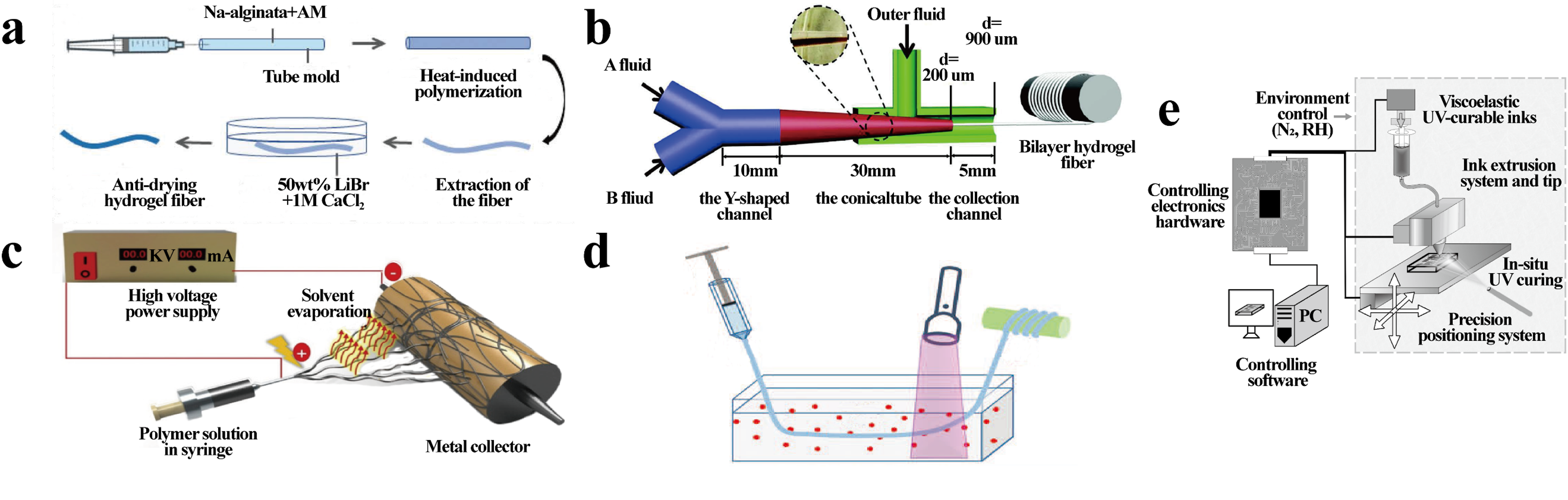
In the past few decades, many researchers have focused their research interests on nanocomposite hydrogel fibers (NHFs). These practitioners have developed and optimized techniques for preparing nanofiber membranes such as the template method, microfluidic spinning, electrospinning, wet spinning and three-dimensional printing (3D printing). NHFs have important applications in wearable monitoring, diagnosis and nursing due to their various excellent properties (such as high-water content, porous morphology, flexibility, braiding and rich active functional groups). In this paper, the latest progress of NHFs in pose monitoring, continuous monitoring of physiological indicators, diagnosis, wearables, nursing, drug delivery and dressings are reviewed. This paper also aims to review their key operational parameters, advantages and disadvantages of NHFs in the above fields, including sensitivity, working range and other special properties. Specifically, NHFs can be used for continuous monitoring of biological postures (such as gestures) or physiological indicators (such as blood sugar) in vitro and in vivo. NHFs also can be used for long-term monitoring of related indicators in the wearable field. NHFs can be used in tissue engineering and drug delivery. Finally, we look forward to the development prospects, challenges and opportunities of the next generation of NHFs. We confirm that the emergence of NHFs in the field of diagnosis and treatment has opened up a new vision for human health. Researchers have optimized the template method, microfluidic spinning, electrospinning, wet spinning and 3D printing.
Citation: Zhenguo Yu, Dong Wang, Zhentan Lu. Nanocomposite hydrogel fibers in the field of diagnosis and treatment[J]. AIMS Materials Science, 2023, 10(6): 1004-1033. doi: 10.3934/matersci.2023054
In the past few decades, many researchers have focused their research interests on nanocomposite hydrogel fibers (NHFs). These practitioners have developed and optimized techniques for preparing nanofiber membranes such as the template method, microfluidic spinning, electrospinning, wet spinning and three-dimensional printing (3D printing). NHFs have important applications in wearable monitoring, diagnosis and nursing due to their various excellent properties (such as high-water content, porous morphology, flexibility, braiding and rich active functional groups). In this paper, the latest progress of NHFs in pose monitoring, continuous monitoring of physiological indicators, diagnosis, wearables, nursing, drug delivery and dressings are reviewed. This paper also aims to review their key operational parameters, advantages and disadvantages of NHFs in the above fields, including sensitivity, working range and other special properties. Specifically, NHFs can be used for continuous monitoring of biological postures (such as gestures) or physiological indicators (such as blood sugar) in vitro and in vivo. NHFs also can be used for long-term monitoring of related indicators in the wearable field. NHFs can be used in tissue engineering and drug delivery. Finally, we look forward to the development prospects, challenges and opportunities of the next generation of NHFs. We confirm that the emergence of NHFs in the field of diagnosis and treatment has opened up a new vision for human health. Researchers have optimized the template method, microfluidic spinning, electrospinning, wet spinning and 3D printing.

| [1] |
Azeem MK, Islam A, Khan RU, et al. (2023) Eco-friendly three-dimensional hydrogels for sustainable agricultural applications: Current and future scenarios. Polym Adv Technol 34: 3046–3062. https://doi.org/10.1002/pat.6122 doi: 10.1002/pat.6122

|
| [2] |
Hou Y, Ma S, Hao J, et al. (2022) Construction and ion transport-related applications of the hydrogel-based membrane with 3D nanochannels. Polymers 14: 4037. https://doi.org/10.3390/polym14194037 doi: 10.3390/polym14194037
|
| [3] |
Matole V, Digge P (2022) A brief review on hydrogel. RJTCS 13: 99–100. https://doi.org/10.52711/2321-5844.2022.00016 doi: 10.52711/2321-5844.2022.00016
|
| [4] |
Ghandforoushan P, Alehosseini M, Golafshan N, et al. (2023) Injectable hydrogels for cartilage and bone tissue regeneration: A review. Int J Biol Macromol 246: 125674. https://doi.org/10.1016/j.ijbiomac.2023.125674 doi: 10.1016/j.ijbiomac.2023.125674
|
| [5] |
Tang Y, Wang H, Liu S, et al. (2022) A review of protein hydrogels: Protein assembly mechanisms, properties, and biological applications. Colloid Surface B 220: 112973. https://doi.org/10.1016/j.colsurfb.2022.112973 doi: 10.1016/j.colsurfb.2022.112973
|
| [6] |
Almajidi YQ, Gupta J, Sheri FS, et al. (2023) Advances in chitosan-based hydrogels for pharmaceutical and biomedical applications: A comprehensive review. Int J Biol Macromol 253: 127278. https://doi.org/10.1016/j.ijbiomac.2023.127278 doi: 10.1016/j.ijbiomac.2023.127278
|
| [7] |
Mahfoudhi N, Boufi S (2016) Poly (acrylic acid-co-acrylamide)/cellulose nanofibrils nanocomposite hydrogels: Effects of CNFs content on the hydrogel properties. Cellulose 23: 3691–3701. https://doi.org/10.1007/s10570-016-1074-z doi: 10.1007/s10570-016-1074-z
|
| [8] |
Chen F, Zhou D, Wang J, et al. (2018) Rational fabrication of anti-freezing, non-drying tough organohydrogels by one-pot solvent displacement. Angew Chem Int Ed 57: 6568–6571. https://doi.org/10.1002/anie.201803366 doi: 10.1002/anie.201803366
|
| [9] |
Sun K, Cui S, Gao X, et al. (2023) Graphene oxide assisted triple network hydrogel electrolyte with high mechanical and temperature stability for self-healing supercapacitor. J Energy Storage 61: 106658. https://doi.org/10.1016/j.est.2023.106658 doi: 10.1016/j.est.2023.106658
|
| [10] |
Bin Asghar Abbasi B, Gigliotti M, Aloko S, et al. (2023) Designing strong, fast, high-performance hydrogel actuators. Chem Commun 59: 7141–7150. https://doi.org/10.1039/D3CC01545A doi: 10.1039/D3CC01545A
|
| [11] |
Wei Z, Gerecht S (2018) A self-healing hydrogel as an injectable instructive carrier for cellular morphogenesis. Biomaterials 185: 86–96. https://doi.org/10.1016/j.biomaterials.2018.09.003 doi: 10.1016/j.biomaterials.2018.09.003
|
| [12] |
Ran C, Wang J, He Y, et al. (2022) Recent advances in bioinspired hydrogels with environment-responsive characteristics for biomedical applications. Macromol Biosci 22: 2100474. https://doi.org/10.1002/mabi.202100474 doi: 10.1002/mabi.202100474
|
| [13] |
Sokolov P, Samokhvalov P, Sukhanova A, et al. (2023) Biosensors based on inorganic composite fluorescent hydrogels. Nanomaterials 13: 1748. https://doi.org/10.3390/nano13111748 doi: 10.3390/nano13111748
|
| [14] |
Su M, Ruan L, Dong X, et al. (2022) Current state of knowledge on intelligent-response biological and other macromolecular hydrogels in biomedical engineering: A review. Int J Biol Macromol 227: 472–492. https://doi.org/10.1016/j.ijbiomac.2022.12.148 doi: 10.1016/j.ijbiomac.2022.12.148
|
| [15] |
Li W, Liu J, Wei J, et al. (2023) Recent progress of conductive hydrogel fibers for flexible electronics: Fabrications, applications, and perspectives. Adv Funct Mater 33: 2213485. https://doi.org/10.1002/adfm.202213485 doi: 10.1002/adfm.202213485
|
| [16] |
Shuai L, Guo ZH, Zhang P, et al. (2020) Stretchable, self-healing, conductive hydrogel fibers for strain sensing and triboelectric energy-harvesting smart textiles. Nano Energy 78: 105389. https://doi.org/10.1016/j.nanoen.2020.105389 doi: 10.1016/j.nanoen.2020.105389
|
| [17] |
Wang XQ, Chan KH, Lu W, et al. (2022) Macromolecule conformational shaping for extreme mechanical programming of polymorphic hydrogel fibers. Nat Commun 13: 3369. https://doi.org/10.1038/s41467-022-31047-3 doi: 10.1038/s41467-022-31047-3
|
| [18] |
Štular D, Kruse M, Župunski V, et al. (2019) Smart stimuli-responsive polylactic acid-hydrogel fibers produced via electrospinning. Fiber Polym 20: 1857–1868. https://doi.org/10.1007/s12221-019-9157-8 doi: 10.1007/s12221-019-9157-8
|
| [19] |
Kim K, Choi JH, Shin M (2021) Mechanical stabilization of alginate hydrogel fiber and 3D constructs by mussel-inspired catechol modification. Polymers 13: 892. https://doi.org/10.3390/polym13060892 doi: 10.3390/polym13060892
|
| [20] |
Luo Y, Shoichet MS (2004) A photolabile hydrogel for guided three-dimensional cell growth and migration. Nat Mater 3: 249–253. https://doi.org/10.1038/nmat1092 doi: 10.1038/nmat1092
|
| [21] |
Du J, Ma Q, Wang B, et al. (2023) Hydrogel fibers for wearable sensors and soft actuators. iScience 26: 106796. https://doi.org/10.1016/j.isci.2023.106796 doi: 10.1016/j.isci.2023.106796
|
| [22] |
Sun W, Zhao X, Webb E, et al. (2023) Advances in metal-organic framework-based hydrogel materials: Preparation, properties and applications. J Mater Chem A 11: 2092–2127. https://doi.org/10.1039/D2TA08841J doi: 10.1039/D2TA08841J
|
| [23] |
Norahan MH, Pedroza-González SC, Sánchez-Salazar MG, et al. (2023) Structural and biological engineering of 3D hydrogels for wound healing. Bioact Mater 24: 197–235. https://doi.org/10.1016/j.bioactmat.2022.11.019 doi: 10.1016/j.bioactmat.2022.11.019
|
| [24] |
Li M, Chen X, Li X, et al. (2021) Wearable and robust polyimide hydrogel fiber textiles for strain sensors. ACS Appl Mater Interfaces 13: 43323–43332. https://doi.org/10.1021/acsami.1c10055 doi: 10.1021/acsami.1c10055
|
| [25] |
Yao B, Wang H, Zhou Q, et al. (2017) Ultrahigh-conductivity polymer hydrogels with arbitrary structures. Adv Mater 29: 1700974. https://doi.org/10.1002/adma.201700974 doi: 10.1002/adma.201700974
|
| [26] |
Rezapour Sarabi M, Jiang N, Ozturk E, et al. (2021) Biomedical optical fibers. Lab Chip 21: 627–640. https://doi.org/10.1039/D0LC01155J doi: 10.1039/D0LC01155J
|
| [27] |
Zaszczyńska A, Niemczyk-Soczynska B, Sajkiewicz P (2022) A comprehensive review of electrospun fibers, 3D-printed scaffolds, and hydrogels for cancer therapies. Polymers 14: 5278. https://doi.org/10.3390/polym14235278 doi: 10.3390/polym14235278
|
| [28] |
Mahaman YAR, Embaye KS, Huang F, et al. (2022) Biomarkers used in Alzheimer's disease diagnosis, treatment, and prevention. Ageing Res Rev 74: 101544. https://doi.org/10.1016/j.arr.2021.101544 doi: 10.1016/j.arr.2021.101544
|
| [29] |
Chen YH, Lou JG, Yang ZH, et al. (2022) Diagnosis, treatment, and prevention of severe acute hepatitis of unknown etiology in children. World J Pediatr 18: 538–544. https://doi.org/10.1007/s12519-022-00581-x doi: 10.1007/s12519-022-00581-x
|
| [30] |
Kher C, Kumar S (2022) The application of nanotechnology and nanomaterials in cancer diagnosis and treatment: A review. Cureus 14: 29059. https://doi.org/10.7759/cureus.29059 doi: 10.7759/cureus.29059
|
| [31] |
Xu W, Qing X, Liu S, et al. (2022) Hollow mesoporous manganese oxides: Application in cancer diagnosis and therapy. Small 18: 2106511. https://doi.org/10.1002/smll.202106511 doi: 10.1002/smll.202106511
|
| [32] |
Song J, Zhang Y, Chan SY, et al. (2021) Hydrogel-based flexible materials for diabetes diagnosis, treatment, and management. Npj Flex Electron 5: 26. https://doi.org/10.1038/s41528-021-00122-y doi: 10.1038/s41528-021-00122-y
|
| [33] |
Li Q, Cao Y, Wang P (2022) Recent advances in hydrogels for the diagnosis and treatment of dry eye disease. Gels 8: 816. https://doi.org/10.3390/gels8120816 doi: 10.3390/gels8120816
|
| [34] |
Zhu JQ, Wu H, Li ZL, et al. (2022) Responsive hydrogels based on triggered click reactions for liver cancer. Adv Mater 34: 2201651. https://doi.org/10.1002/adma.202201651 doi: 10.1002/adma.202201651
|
| [35] |
Ma Y, Huang J, Song S, et al. (2016) Cancer-targeted nanotheranostics: Recent advances and perspectives. Small 12: 4936–4954. https://doi.org/10.1002/smll.201600635 doi: 10.1002/smll.201600635
|
| [36] |
Tehrany PM, Rahmanian P, Rezaee A, et al. (2023) Multifunctional and theranostic hydrogels for wound healing acceleration: An emphasis on diabetic-related chronic wounds. Environ Res 238: 117087. https://doi.org/10.1016/j.envres.2023.117087 doi: 10.1016/j.envres.2023.117087
|
| [37] |
Gupta BD, Pathak A, Shrivastav AM (2022) Optical biomedical diagnostics using lab-on-fiber technology: A review. Photonics 9: 86. https://doi.org/10.3390/photonics9020086 doi: 10.3390/photonics9020086
|
| [38] |
Zhou C, Wu T, Xie X, et al. (2022) Advances and challenges in conductive hydrogels: From properties to applications. Eur Polym J 177: 111454. https://doi.org/10.1016/j.eurpolymj.2022.111454 doi: 10.1016/j.eurpolymj.2022.111454
|
| [39] |
Liu Y, Wang L, Mi Y, et al. (2022) Transparent stretchable hydrogel sensors: Materials, design and applications. J Mater Chem C 10: 13351–13371. https://doi.org/10.1039/D2TC01104B doi: 10.1039/D2TC01104B
|
| [40] |
Liu G, Chen X, Zhou W, et al. (2016) Preparation of a novel composite nanofiber gel‑encapsulated human placental extract through layer‑by‑layer self‑assembly. Exp Ther Med 11: 1447–1452. https://doi.org/10.3892/etm.2016.3084 doi: 10.3892/etm.2016.3084
|
| [41] |
Zhao Z, Fang R, Rong Q, et al. (2017) Bioinspired nanocomposite hydrogels with highly ordered structures. Adv Mater 29: 1703045. https://doi.org/10.1002/adma.201703045 doi: 10.1002/adma.201703045
|
| [42] |
Li J, Li S, Huang J, et al. (2022) Spider silk-inspired artificial fibers. Adv Sci 9: 2103965. https://doi.org/10.1002/advs.202103965 doi: 10.1002/advs.202103965
|
| [43] |
Zhang X, Wang X, Fan W, et al. (2022) Fabrication, property and application of calcium alginate fiber: A review. Polymers 14: 3227. https://doi.org/10.3390/polym14153227 doi: 10.3390/polym14153227
|
| [44] |
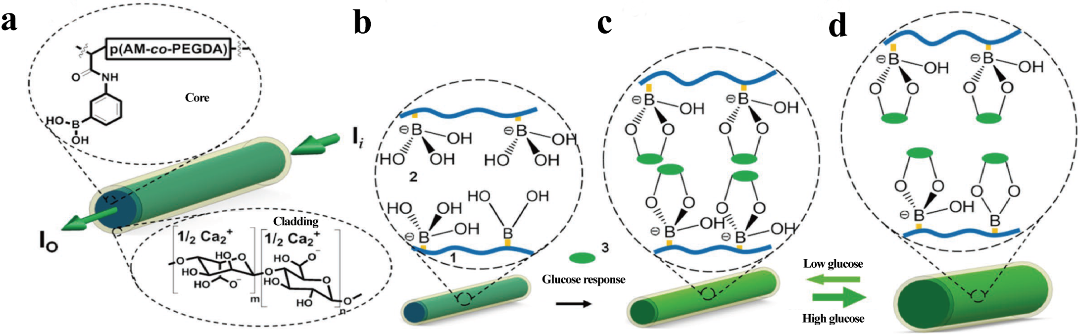
Yetisen AK, Jiang N, Fallahi A, et al. (2017) Glucose-sensitive hydrogel optical fibers functionalized with phenylboronic acid. Adv Mater 29: 1606380. https://doi.org/10.1002/adma.201606380 doi: 10.1002/adma.201606380
|
| [45] |
Choi M, Humar M, Kim S, et al. (2015) Step-index optical fiber made of biocompatible hydrogels. Adv Mater 27: 4081–4086. https://doi.org/10.1002/adma.201501603 doi: 10.1002/adma.201501603
|
| [46] |
Zhang S, Chen Y, Liu H, et al. (2020) Room-temperature-formed PEDOT:PSS hydrogels enable injectable, soft, and healable organic bioelectronics. Adv Mater 32: 1904752. https://doi.org/10.1002/adma.201904752 doi: 10.1002/adma.201904752
|
| [47] |
Li Y, Poon CT, Li M, et al. (2015) Chinese-noodle-inspired muscle myofiber fabrication. Adv Funct Mater 25: 5999–6008. https://doi.org/10.1002/adfm.201502018 doi: 10.1002/adfm.201502018
|
| [48] |
Dou Y, Wang ZP, He W, et al. (2019) Artificial spider silk from ion-doped and twisted core-sheath hydrogel fibres. Nat Commun 10: 5293. https://doi.org/10.1038/s41467-019-13257-4 doi: 10.1038/s41467-019-13257-4
|
| [49] |
Kim SH, Kim SH, Nair S, et al. (2005) Reactive electrospinning of cross-linked poly(2-hydroxyethyl methacrylate) nanofibers and elastic properties of individual hydrogel nanofibers in aqueous solutions. Macromolecules 38: 3719–3723. https://doi.org/10.1021/ma050308g doi: 10.1021/ma050308g
|
| [50] |
Jeong W, Kim J, Kim S, et al. (2004) Hydrodynamic microfabrication via "on the fly" photopolymerization of microscale fibers and tubes. Lab Chip 4: 576–580. https://doi.org/10.1039/B411249K doi: 10.1039/B411249K
|
| [51] |
Scotti A, Schulte MF, Lopez CG, et al. (2022) How softness matters in soft nanogels and nanogel assemblies. Chem Rev 122: 11675–11700. https://doi.org/10.1021/acs.chemrev.2c00035 doi: 10.1021/acs.chemrev.2c00035
|
| [52] |
Ko A, Liao C (2023) Hydrogel wound dressings for diabetic foot ulcer treatment: Status-quo, challenges, and future perspectives. BMEMat 1: e12037. https://doi.org/10.1002/bmm2.12037 doi: 10.1002/bmm2.12037
|
| [53] |
Li P, Jin Z, Peng L, et al. (2018) Stretchable all-gel-state fiber-shaped supercapacitors enabled by macromolecularly interconnected 3D graphene/nanostructured conductive polymer hydrogels. Adv Mater 30: 1800124. https://doi.org/10.1002/adma.201800124 doi: 10.1002/adma.201800124
|
| [54] |
Perazzo A, Nunes JK, Guido S, et al. (2017) Flow-induced gelation of microfiber suspensions. P Natl Acad Sci USA 114: E8557–E8564. https://doi.org/10.1073/pnas.1710927114 doi: 10.1073/pnas.1710927114
|
| [55] |
Kim J, Kang T, Kim H, et al. (2019) Preparation of PVA/PAA nanofibers containing thiol-modified silica particles by electrospinning as an eco-friendly Cu (Ⅱ) adsorbent. J Ind Eng Chem 77: 273–279. https://doi.org/10.1016/j.jiec.2019.04.048 doi: 10.1016/j.jiec.2019.04.048
|
| [56] |
Cui Q, Bell DJ, Rauer SB, et al. (2020) Wet-spinning of biocompatible core-shell polyelectrolyte complex fibers for tissue engineering. Adv Mater Interfaces 7: 2000849. https://doi.org/10.1002/admi.202000849 doi: 10.1002/admi.202000849
|
| [57] |
Jin Y, Liu C, Chai W, et al. (2017) Self-supporting nanoclay as internal scaffold material for direct printing of soft hydrogel composite structures in air. ACS Appl Mater Interfaces 9: 17456–17465. https://doi.org/10.1021/acsami.7b03613 doi: 10.1021/acsami.7b03613
|
| [58] |
Foudazi R, Zowada R, Manas-Zloczower I, et al. (2023) Porous hydrogels: Present challenges and future opportunities. Langmuir 39: 2092–2111. https://doi.org/10.1021/acs.langmuir.2c02253 doi: 10.1021/acs.langmuir.2c02253
|
| [59] |
Tamayol A, Najafabadi AH, Aliakbarian B, et al. (2015) Hydrogel templates for rapid manufacturing of bioactive fibers and 3D constructs. Adv Healthc Mater 4: 2146–2153. https://doi.org/10.1002/adhm.201500492 doi: 10.1002/adhm.201500492
|
| [60] |
Ding H, Wu Z, Wang H, et al. (2022) An ultrastretchable, high-performance, and crosstalk-free proximity and pressure bimodal sensor based on ionic hydrogel fibers for human-machine interfaces. Mater Horiz 9: 1935–1946. https://doi.org/10.1039/D2MH00281G doi: 10.1039/D2MH00281G
|
| [61] |
Yin T, Wu L, Wu T, et al. (2019) Ultrastretchable and conductive core/sheath hydrogel fibers with multifunctionality. J Polym Sci Part B: Polym Phys 57: 272–280. https://doi.org/10.1002/polb.24781 doi: 10.1002/polb.24781
|
| [62] |
Wang L, Zhong C, Ke D, et al. (2018) Ultrasoft and highly stretchable hydrogel optical fibers for in vivo optogenetic modulations. Adv Opt Mater 6: 1800427. https://doi.org/10.1002/adom.201800427 doi: 10.1002/adom.201800427
|
| [63] |
Cheng J, Jun Y, Qin J, et al. (2017) Electrospinning versus microfluidic spinning of functional fibers for biomedical applications. Biomaterials 114: 121–143. https://doi.org/10.1016/j.biomaterials.2016.10.040 doi: 10.1016/j.biomaterials.2016.10.040
|
| [64] |
Ahn SY, Mun CH, Lee SH (2015) Microfluidic spinning of fibrous alginate carrier having highly enhanced drug loading capability and delayed release profile. RSC Adv 5: 15172–15181. https://doi.org/10.1039/C4RA11438H doi: 10.1039/C4RA11438H
|
| [65] |
Zhou M, Gong J, Ma J (2019) Continuous fabrication of near-infrared light responsive bilayer hydrogel fibers based on microfluidic spinning. E-Polymers 19: 215–224. https://doi.org/10.1515/epoly-2019-0022 doi: 10.1515/epoly-2019-0022
|
| [66] |
Shi X, Ostrovidov S, Zhao Y, et al. (2015) Microfluidic spinning of cell-responsive grooved microfibers. Adv Funct Mater 25: 2250–2259. https://doi.org/10.1002/adfm.201404531 doi: 10.1002/adfm.201404531
|
| [67] | Kasper FK, Liao J, Kretlow JD, et al. (1979) Flow Perfusion Culture of Mesenchymal Stem Cells for Bone Tissue Engineering, Cambridge: Harvard Stem Cell Institute. https://doi.org/10.3824/stembook.1.18.1 |
| [68] |
Gao Z, Xiao X, Carlo AD, et al. (2023) Advances in wearable strain sensors based on electrospun fibers. Adv Funct Mater 33: 2214265. https://doi.org/10.1002/adfm.202214265 doi: 10.1002/adfm.202214265
|
| [69] |
Chen C, Tang J, Gu Y, et al. (2019) Bioinspired hydrogel electrospun fibers for spinal cord regeneration. Adv Funct Mater 29: 1806899. https://doi.org/10.1002/adfm.201806899 doi: 10.1002/adfm.201806899
|
| [70] |
Im JS, Bai BC, In SJ, et al. (2010) Improved photodegradation properties and kinetic models of a solar-light-responsive photocatalyst when incorporated into electrospun hydrogel fibers. J Colloid Interf Sci 346: 216–221. https://doi.org/10.1016/j.jcis.2010.02.043 doi: 10.1016/j.jcis.2010.02.043
|
| [71] |
Han F, Zhang H, Zhao J, et al. (2012) In situ encapsulation of hydrogel in ultrafine fibers by suspension electrospinning. Polym Eng Sci 52: 2695–2704. https://doi.org/10.1002/pen.23227 doi: 10.1002/pen.23227
|
| [72] |
Mirabedini A, Foroughi J, Romeo T, et al. (2015) Development and characterization of novel hybrid hydrogel fibers. Macromol Mater Eng 300: 1217–1225. https://doi.org/10.1002/mame.201500152 doi: 10.1002/mame.201500152
|
| [73] |
Song JC, Chen S, Sun LJ, et al. (2020) Mechanically and electronically robust transparent organohydrogel fibers. Adv Mater 32: 1906994. https://doi.org/10.1002/adma.201906994 doi: 10.1002/adma.201906994
|
| [74] |
Nechyporchuk O, Yang Nilsson T, Ulmefors H, et al. (2020) Wet spinning of chitosan fibers: Effect of sodium dodecyl sulfate adsorption and enhanced dope temperature. ACS Appl Polym Mater 2: 3867–3875. https://doi.org/10.1021/acsapm.0c00562 doi: 10.1021/acsapm.0c00562
|
| [75] |
Konop AJ, Colby RH (1999) Polyelectrolyte charge effects on solution viscosity of poly(acrylic acid). Macromolecules 32: 2803–2805. https://doi.org/10.1021/ma9818174 doi: 10.1021/ma9818174
|
| [76] |
Li S, Biswas MC, Ford E (2022) Dual roles of sodium polyacrylate in alginate fiber wet-spinning: Modify the solution rheology and strengthen the fiber. Carbohyd Polym 297: 120001. https://doi.org/10.1016/j.carbpol.2022.120001 doi: 10.1016/j.carbpol.2022.120001
|
| [77] |
He Y, Zhang N, Gong Q, et al. (2012) Alginate/graphene oxide fibers with enhanced mechanical strength prepared by wet spinning. Carbohyd Polym 88: 1100–1108. https://doi.org/10.1016/j.carbpol.2012.01.071 doi: 10.1016/j.carbpol.2012.01.071
|
| [78] |
Zhang C, Xiao P, Zhang D, et al. (2023) Wet-spinning knittable hygroscopic organogel fibers toward moisture-capture-enabled multifunctional devices. Adv Fiber Mater 5: 588–602. https://doi.org/10.1007/s42765-022-00243-7 doi: 10.1007/s42765-022-00243-7
|
| [79] |
Sharma A, Ansari MZ, Cho C (2022) Ultrasensitive flexible wearable pressure/strain sensors: Parameters, materials, mechanisms and applications. Sensor Actuat A-Phys 347: 113934. https://doi.org/10.1016/j.sna.2022.113934 doi: 10.1016/j.sna.2022.113934
|
| [80] |
Nasiri S, Khosravani MR (2020) Progress and challenges in fabrication of wearable sensors for health monitoring. Sensor Actuat A-Phys 312: 112105. https://doi.org/10.1016/j.sna.2020.112105 doi: 10.1016/j.sna.2020.112105
|
| [81] |
Tian K, Bae J, Bakarich SE, et al. (2017) 3D printing of transparent and conductive heterogeneous hydrogel-elastomer systems. Adv Mater 29: 1604827. https://doi.org/10.1002/adma.201604827 doi: 10.1002/adma.201604827
|
| [82] |
Liu C, Wang Z, Wei X, et al. (2021) 3D printed hydrogel/PCL core/shell fiber scaffolds with NIR-triggered drug release for cancer therapy and wound healing. Acta Biomater 131: 314–325. https://doi.org/10.1016/j.actbio.2021.07.011 doi: 10.1016/j.actbio.2021.07.011
|
| [83] |
Zheng SY, Shen Y, Zhu F, et al. (2018) Programmed deformations of 3D-printed tough physical hydrogels with high response speed and large output force. Adv Funct Mater 28: 1803366. https://doi.org/10.1002/adfm.201803366 doi: 10.1002/adfm.201803366
|
| [84] |
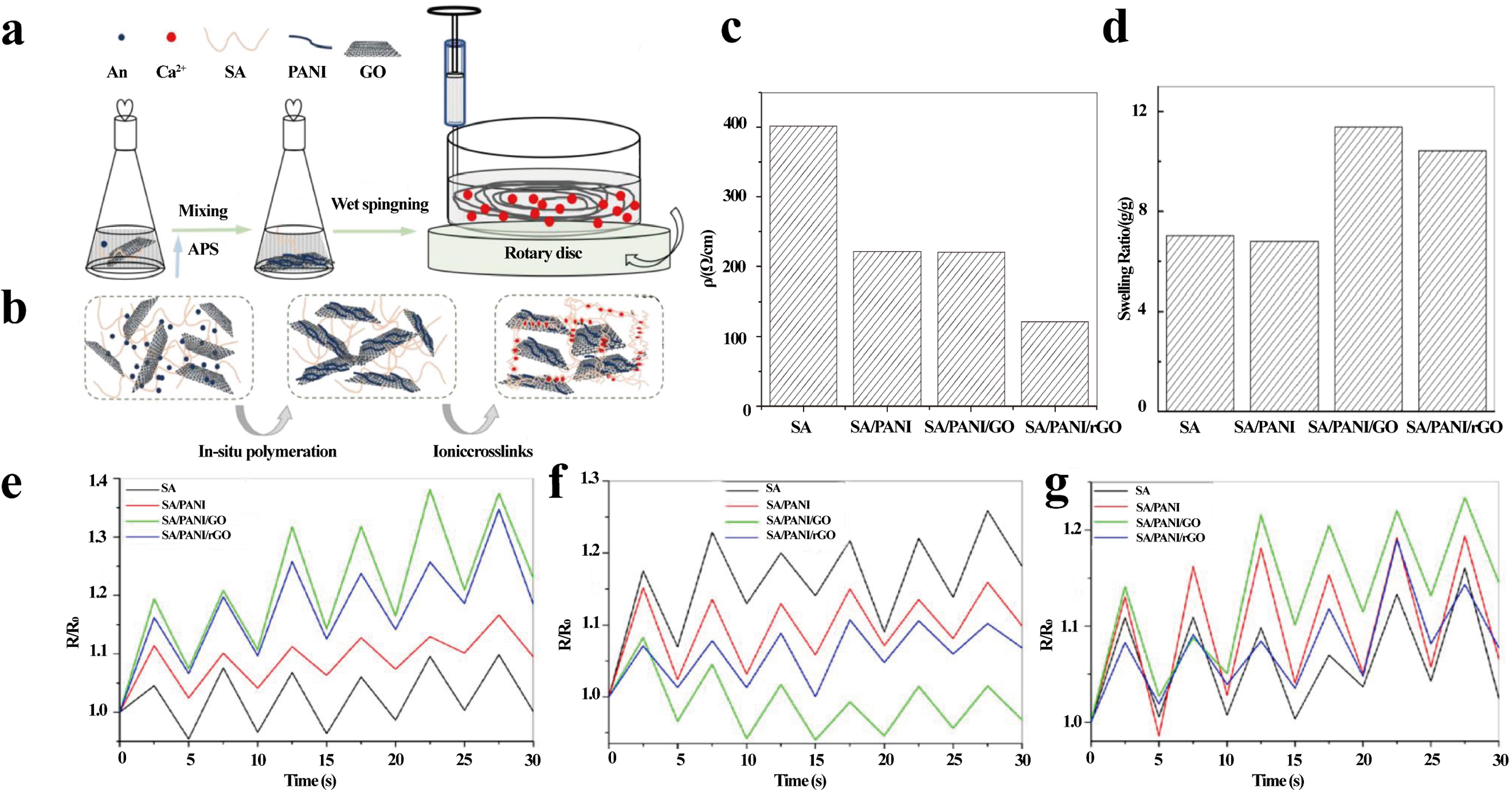
Wu Y, Zhou S, Yi J, et al. (2022) Facile fabrication of flexible alginate/polyaniline/graphene hydrogel fibers for strain sensor. J Eng Fiber Fabr 17. https://doi.org/10.1177/15589250221114641 doi: 10.1177/15589250221114641
|
| [85] |
Guo J, Liu X, Jiang N, et al. (2016) Highly stretchable, strain sensing hydrogel optical fibers. Adv Mater 28: 10244–10249. https://doi.org/10.1002/adma.201603160 doi: 10.1002/adma.201603160
|
| [86] |
Shi W, Wang Z, Song H, et al. (2022) High-sensitivity and extreme environment-resistant sensors based on PEDOT:PSS@PVA hydrogel fibers for physiological monitoring. ACS Appl Mater Interfaces 14: 35114–35125. https://doi.org/10.1021/acsami.2c09556 doi: 10.1021/acsami.2c09556
|
| [87] |
Mian Z, Hermayer KL, Jenkins A (2019) Continuous glucose monitoring: Review of an innovation in diabetes management. Am J Med Sci 358: 332–339. https://doi.org/10.1016/j.amjms.2019.07.003 doi: 10.1016/j.amjms.2019.07.003
|
| [88] |
Xie Y, Lu L, Gao F, et al. (2021) Integration of artificial intelligence, blockchain, and wearable technology for chronic disease management: A new paradigm in smart healthcare. Curr Med Sci 41: 1123–1133. https://doi.org/10.1007/s11596-021-2485-0 doi: 10.1007/s11596-021-2485-0
|
| [89] |
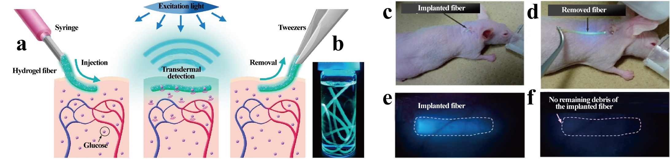
Heo YJ, Shibata H, Okitsu T, et al. (2011) Long-term in vivo glucose monitoring using fluorescent hydrogel fibers. P Natl Acad Sci USA 108: 13399–13403. https://doi.org/10.1073/pnas.1104954108 doi: 10.1073/pnas.1104954108
|
| [90] | Heo YJ, Shibata H, Okitsu T, et al. (2011) Fluorescent hydrogel fibers for long-term in vivo glucose monitoring. 16th International Solid-State Sensors, Actuators and Microsystems Conference, Beijing, China, 2140–214. https://10.1109/TRANSDUCERS.2011.5969342 |
| [91] |
Nunoi H, Xie P, Nakamura H, et al. (2022) Treatment with polyethylene glycol-conjugated fungal d-amino acid oxidase reduces lung inflammation in a mouse model of chronic granulomatous disease. Inflammation 45: 1668–1679. https://doi.org/10.1007/s10753-022-01650-z doi: 10.1007/s10753-022-01650-z
|
| [92] |
Besir Y, Karaagac E, Kurus M, et al. (2023) The effect of bovine serum albumin-glutaraldehyde and polyethylene glycol polymer on local tissue reaction and inflammation in rabbit carotid artery anastomosis. Vascular 31: 554–563. https://doi.org/10.1177/17085381221075484 doi: 10.1177/17085381221075484
|
| [93] |
Zdolsek J, Eaton JW, Tang L (2007) Histamine release and fibrinogen adsorption mediate acute inflammatory responses to biomaterial implants in humans. J Transl Med 5: 31. https://doi.org/10.1186/1479-5876-5-31 doi: 10.1186/1479-5876-5-31
|
| [94] |
Bosetti M, Zanardi L, Bracco P, et al. (2003) In vitro evaluation of the inflammatory activity of ultra-high molecular weight polyethylene. Biomaterials 24: 1419–1426. https://doi.org/10.1016/S0142-9612(02)00526-4 doi: 10.1016/S0142-9612(02)00526-4
|
| [95] |
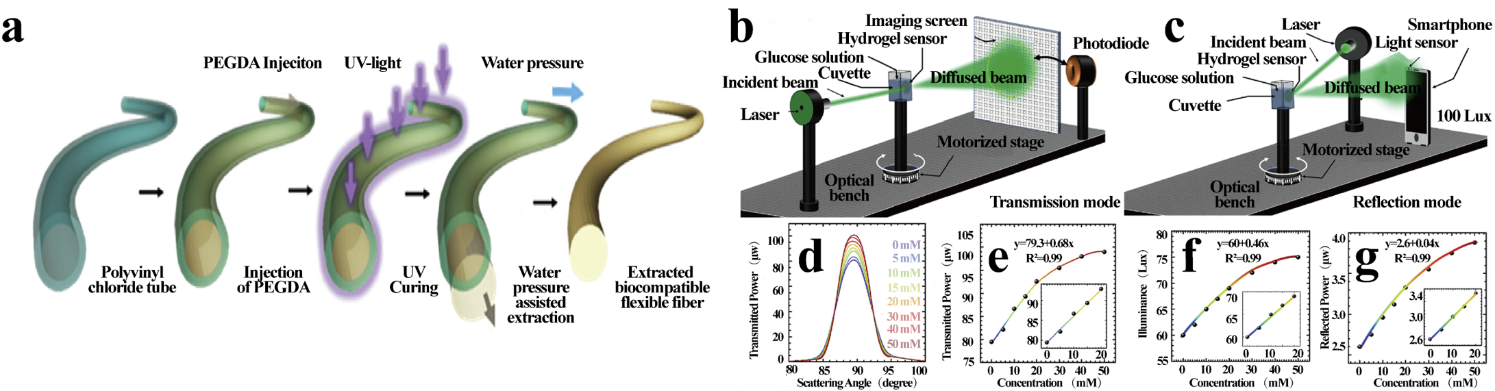
Elsherif M, Hassan MU, Yetisen AK, et al. (2019) Hydrogel optical fibers for continuous glucose monitoring. Biosens Bioelectron 137: 25–32. https://doi.org/10.1016/j.bios.2019.05.002 doi: 10.1016/j.bios.2019.05.002
|
| [96] |
De Fazio R, De Vittorio M, Visconti P (2021) Innovative IoT solutions and wearable sensing systems for monitoring human biophysical parameters: A review. Electronics 10: 1660. https://doi.org/10.3390/electronics10141660 doi: 10.3390/electronics10141660
|
| [97] |
Seshadri DR, Li RT, Voos JE, et al. (2019) Wearable sensors for monitoring the physiological and biochemical profile of the athlete. NPJ Digit Med 2: 72. https://doi.org/10.1038/s41746-019-0150-9 doi: 10.1038/s41746-019-0150-9
|
| [98] |
Bandodkar AJ, Jeang WJ, Ghaffari R, et al. (2019) Wearable sensors for biochemical sweat analysis. Annu Rev Anal Chem 12: 1–22. https://doi.org/10.1146/annurev-anchem-061318-114910 doi: 10.1146/annurev-anchem-061318-114910
|
| [99] |
Hanlon M, Anderson R (2009) Real-time gait event detection using wearable sensors. Gait Posture 30: 523–527. https://doi.org/10.1016/j.gaitpost.2009.07.128 doi: 10.1016/j.gaitpost.2009.07.128
|
| [100] |
Prasanth H, Caban M, Keller U, et al. (2021) Wearable sensor-based real-time gait detection: A systematic review. Sensors 21: 2727. https://doi.org/10.3390/s21082727 doi: 10.3390/s21082727
|
| [101] |
Wan F, Ping H, Wang W, et al. (2021) Hydroxyapatite-reinforced alginate fibers with bioinspired dually aligned architectures. Carbohyd Polym 267: 118167. https://doi.org/10.1016/j.carbpol.2021.118167 doi: 10.1016/j.carbpol.2021.118167
|
| [102] |
Duan X, Yu J, Zhu Y, et al. (2020) Large-scale spinning approach to engineering knittable hydrogel fiber for soft robots. ACS Nano 14: 14929–14938. https://doi.org/10.1021/acsnano.0c04382 doi: 10.1021/acsnano.0c04382
|
| [103] |
Song J, Chen S, Sun L, et al. (2020) Mechanically and electronically robust transparent organohydrogel fibers. Adv Mater 32: 1906994. https://doi.org/10.1002/adma.201906994 doi: 10.1002/adma.201906994
|
| [104] |
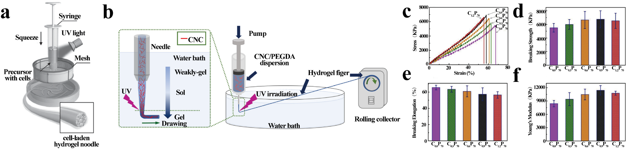
Hou K, Li Y, Liu Y, et al. (2017) Continuous fabrication of cellulose nanocrystal/poly(ethylene glycol) diacrylate hydrogel fiber from nanocomposite dispersion: Rheology, preparation and characterization. Polymer 123: 55–64. https://doi.org/10.1016/j.polymer.2017.06.034 doi: 10.1016/j.polymer.2017.06.034
|
| [105] |
Dzenis Y (2004) Spinning continuous fibers for nanotechnology. Science 304: 1917–1919. https://www.science.org/doi/10.1126/science.1099074 doi: 10.1126/science.1099074
|
| [106] |
Zhao L, Xu T, Wang B, et al. (2023) Continuous fabrication of robust ionogel fibers for ultrastable sensors via dynamic reactive spinning. Chem Eng J 455: 140796. https://doi.org/10.1016/j.cej.2022.140796 doi: 10.1016/j.cej.2022.140796
|
| [107] |
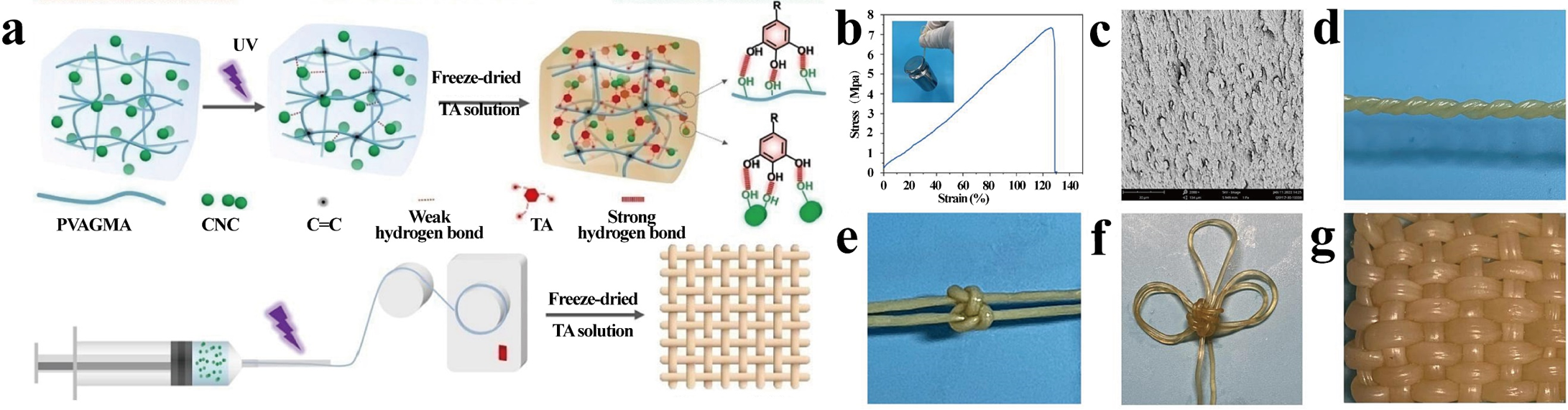
Pei M, Zhu D, Yang J, et al. (2023) Multi-crosslinked flexible nanocomposite hydrogel fibers with excellent strength and knittability. Eur Polym J 182: 111737. https://doi.org/10.1016/j.eurpolymj.2022.111737 doi: 10.1016/j.eurpolymj.2022.111737
|
| [108] |
Hua J, Liu C, Fei B, et al. (2022) Self-healable and super-tough double-network hydrogel fibers from dynamic acylhydrazone bonding and supramolecular interactions. Gels 8: 101. https://doi.org/10.3390/gels8020101 doi: 10.3390/gels8020101
|
| [109] |
Wang C, Zhai S, Yuan Z, et al. (2020) Drying graphene hydrogel fibers for capacitive energy storage. Carbon 164: 100–110. https://doi.org/10.1016/j.carbon.2020.03.053 doi: 10.1016/j.carbon.2020.03.053
|
| [110] |
Meng F, Ding Y (2011) Sub-micrometer-thick all-solid-state supercapacitors with high power and energy densities. Adv Mater 23: 4098–4102. https://doi.org/10.1002/adma.201101678 doi: 10.1002/adma.201101678
|
| [111] |
Yang B, Hao C, Wen F, et al. (2017) Flexible black-phosphorus nanoflake/carbon nanotube composite paper for high-performance all-solid-state supercapacitors. ACS Appl Mater Interfaces 9: 44478–44484. https://doi.org/10.1021/acsami.7b13572 doi: 10.1021/acsami.7b13572
|
| [112] |
Zhang X, Chen Y, Yan J, et al. (2020) Janus-faced film with dual function of conductivity and pseudo-capacitance for flexible supercapacitors with ultrahigh energy density. Chem Eng J 388: 124197. https://doi.org/10.1016/j.cej.2020.124197 doi: 10.1016/j.cej.2020.124197
|
| [113] |
Han X, Xiao G, Wang Y, et al. (2020) Design and fabrication of conductive polymer hydrogels and their applications in flexible supercapacitors. J Mater Chem A 8: 23059–23095. https://doi.org/10.1039/D0TA07468C doi: 10.1039/D0TA07468C
|
| [114] |
Huang H, Han L, Fu X, et al. (2021) A powder self-healable hydrogel electrolyte for flexible hybrid supercapacitors with high energy density and sustainability. Small 17: 2006807. https://doi.org/10.1002/smll.202006807 doi: 10.1002/smll.202006807
|
| [115] |
Jia R, Li L, Ai Y, et al. (2018) Self-healable wire-shaped supercapacitors with two twisted NiCo2O4 coated polyvinyl alcohol hydrogel fibers. Sci China Mater 61: 254–262. https://doi.org/10.1007/s40843-017-9177-5 doi: 10.1007/s40843-017-9177-5
|
| [116] |
Xu T, Yang D, Zhang S, et al. (2021) Antifreezing and stretchable all-gel-state supercapacitor with enhanced capacitances established by graphene/PEDOT-polyvinyl alcohol hydrogel fibers with dual networks. Carbon 171: 201–210. https://doi.org/10.1016/j.carbon.2020.08.071 doi: 10.1016/j.carbon.2020.08.071
|
| [117] |
Cao X, Jiang C, Sun N, et al. (2021) Recent progress in multifunctional hydrogel-based supercapacitors. J Sci-Adv Mater Dev 6: 338–350. https://doi.org/10.1016/j.jsamd.2021.06.002 doi: 10.1016/j.jsamd.2021.06.002
|
| [118] |
Liu J, Jia Y, Jiang Q, et al. (2018) Highly conductive hydrogel polymer fibers toward promising wearable thermoelectric energy harvesting. ACS Appl Mater Interfaces 10: 44033–44040. https://doi.org/10.1021/acsami.8b15332 doi: 10.1021/acsami.8b15332
|
| [119] |
Zhou M, Al-Furjan MSH, Zou J, et al. (2018) A review on heat and mechanical energy harvesting from human-principles, prototypes and perspectives. Renew Sust Energ Rev 82: 3582–3609. https://doi.org/10.1016/j.rser.2017.10.102 doi: 10.1016/j.rser.2017.10.102
|
| [120] |
Huang L, Lin S, Xu Z, et al. (2020) Fiber-based energy conversion devices for human-body energy harvesting. Adv Mater 32: 1902034. https://doi.org/10.1002/adma.201902034 doi: 10.1002/adma.201902034
|
| [121] |
Peng L, Liu Y, Huang J, et al. (2018) Microfluidic fabrication of highly stretchable and fast electro-responsive graphene oxide/polyacrylamide/alginate hydrogel fibers. Eur Polym J 103: 335–341. https://doi.org/10.1016/j.eurpolymj.2018.04.019 doi: 10.1016/j.eurpolymj.2018.04.019
|
| [122] |
Wang Y, Ding Y, Guo X, et al. (2019) Conductive polymers for stretchable supercapacitors. Nano Res 12: 1978–1987. https://doi.org/10.1007/s12274-019-2296-9 doi: 10.1007/s12274-019-2296-9
|
| [123] |
Zhao X, Chen F, Li Y, et al. (2018) Bioinspired ultra-stretchable and anti-freezing conductive hydrogel fibers with ordered and reversible polymer chain alignment. Nat Commun 9: 3579. https://doi.org/10.1038/s41467-018-05904-z doi: 10.1038/s41467-018-05904-z
|
| [124] |
Bai J, Liu D, Tian X, et al. (2022) Tissue-like organic electrochemical transistors. J Mater Chem C 10: 13303–13311. https://doi.org/10.1039/D2TC01530G doi: 10.1039/D2TC01530G
|
| [125] |
Kayser LV, Lipomi DJ (2019) Stretchable conductive polymers and composites based on PEDOT and PEDOT:PSS. Adv Mater 31: 1806133. https://doi.org/10.1002/adma.201806133 doi: 10.1002/adma.201806133
|
| [126] |
Tseghai GB, Mengistie DA, Malengier B, et al. (2020) PEDOT:PSS-based conductive textiles and their applications. Sensors 20: 1881. https://doi.org/10.3390/s20071881 doi: 10.3390/s20071881
|
| [127] |
Zhao P, Zhang R, Tong Y, et al. (2020) Strain-discriminable pressure/proximity sensing of transparent stretchable electronic skin based on PEDOT:PSS/SWCNT electrodes. ACS Appl Mater Interfaces 12: 55083–55093. https://doi.org/10.1021/acsami.0c16546 doi: 10.1021/acsami.0c16546
|
| [128] |
Li P, Wang Y, Gupta U, et al. (2019) Transparent soft robots for effective camouflage. Adv Funct Mater 29: 1901908. https://doi.org/10.1002/adfm.201901908 doi: 10.1002/adfm.201901908
|
| [129] |
Li Y, Wang J, Wang Y, et al. (2021) Advanced electrospun hydrogel fibers for wound healing. Compos Part B-Eng 223: 109101. https://doi.org/10.1016/j.compositesb.2021.109101 doi: 10.1016/j.compositesb.2021.109101
|
| [130] |
Neibert K, Gopishetty V, Grigoryev A, et al. (2012) Wound-healing with mechanically robust and biodegradable hydrogel fibers loaded with silver nanoparticles. Adv Healthc Mater 1: 621–630. https://doi.org/10.1002/adhm.201200075 doi: 10.1002/adhm.201200075
|
| [131] |
Peng J, Cheng Q (2017) High-performance nanocomposites inspired by nature. Adv Mater 29: 1702959. https://doi.org/10.1002/adma.201702959 doi: 10.1002/adma.201702959
|
| [132] |
Xia LW, Xie R, Ju XJ, et al. (2013) Nano-structured smart hydrogels with rapid response and high elasticity. Nat Commun 4: 2226. https://doi.org/10.1038/ncomms3226 doi: 10.1038/ncomms3226
|
| [133] |
Lan Z, Kar R, Chwatko M, et al. (2023) High porosity PEG-based hydrogel foams with self-tuning moisture balance as chronic wound dressings. J Biomed Mater Res A 111: 465–477. https://doi.org/10.1002/jbm.a.37498 doi: 10.1002/jbm.a.37498
|
| [134] |
Farahani M, Shafiee A (2021) Wound healing: From passive to smart dressings. Adv Healthc Mater 10: 2100477. https://doi.org/10.1002/adhm.202100477 doi: 10.1002/adhm.202100477
|
| [135] |
Zhang Q, Qian C, Xiao W, et al. (2019) Development of a visible light, cross-linked GelMA hydrogel containing decellularized human amniotic particles as a soft tissue replacement for oral mucosa repair. RSC Adv 9: 18344–18352. https://doi.org/10.1039/C9RA03009C doi: 10.1039/C9RA03009C
|
| [136] |
Raho R, Paladini F, Lombardi FA, et al. (2015) In-situ photo-assisted deposition of silver particles on hydrogel fibers for antibacterial applications. Mater Sci Eng C 55: 42–49. https://doi.org/10.1016/j.msec.2015.05.050 doi: 10.1016/j.msec.2015.05.050
|
| [137] |
Ji Y, Ghosh K, Li B, et al. (2006) Dual-syringe reactive electrospinning of cross-linked hyaluronic acid hydrogel nanofibers for tissue engineering applications. Macromol Biosci 6: 811–817. https://doi.org/10.1002/mabi.200600132 doi: 10.1002/mabi.200600132
|
| [138] |
Sun X, Lang Q, Zhang H, et al. (2017) Electrospun photocrosslinkable hydrogel fibrous scaffolds for rapid in vivo vascularized skin flap regeneration. Adv Funct Mater 27: 1604617. https://doi.org/10.1002/adfm.201604617 doi: 10.1002/adfm.201604617
|
| [139] |
Liu W, Bi W, Sun Y, et al. (2020) Biomimetic organic-inorganic hybrid hydrogel electrospinning periosteum for accelerating bone regeneration. Mater Sci Eng C 110: 110670. https://doi.org/10.1016/j.msec.2020.110670 doi: 10.1016/j.msec.2020.110670
|
| [140] |
Wei X, Liu C, Wang Z, et al. (2020) 3D printed core-shell hydrogel fiber scaffolds with NIR-triggered drug release for localized therapy of breast cancer. Int J Pharm 580: 119219. https://doi.org/10.1016/j.ijpharm.2020.119219 doi: 10.1016/j.ijpharm.2020.119219
|
| [141] |
Tsourdi E, Barthel A, Rietzsch H, et al. (2013) Current aspects in the pathophysiology and treatment of chronic wounds in diabetes mellitus. Biomed Res Int 2013: 385641. https://doi.org/10.1155/2013/385641 doi: 10.1155/2013/385641
|
| [142] |
Chen H, Jia P, Kang H, et al. (2016) Upregulating hif-1α by hydrogel nanofibrous scaffolds for rapidly recruiting angiogenesis relative cells in diabetic wound. Adv Healthc Mater 5: 907–918. https://doi.org/10.1002/adhm.201501018 doi: 10.1002/adhm.201501018
|
| [143] |
Zhou P, Zhou L, Zhu C, et al. (2016) Nanogel-electrospinning for controlling the release of water-soluble drugs. J Mater Chem B 4: 2171–2178. https://doi.org/10.1039/C6TB00023A doi: 10.1039/C6TB00023A
|
| [144] |
Zhao X, Sun X, Yildirimer L, et al. (2017) Cell infiltrative hydrogel fibrous scaffolds for accelerated wound healing. Acta Biomater 49: 66–77. https://doi.org/10.1016/j.actbio.2016.11.017 doi: 10.1016/j.actbio.2016.11.017
|
| [145] |
Wang H, Xu Z, Zhao M, et al. (2021) Advances of hydrogel dressings in diabetic wounds. Biomater Sci 9: 1530–1546. https://doi.org/10.1039/D0BM01747G doi: 10.1039/D0BM01747G
|
| [146] |
Lei H, Zhu C, Fan D (2020) Optimization of human-like collagen composite polysaccharide hydrogel dressing preparation using response surface for burn repair. Carbohyd Polym 239: 116249. https://doi.org/10.1016/j.carbpol.2020.116249 doi: 10.1016/j.carbpol.2020.116249
|
| [147] |
Kesharwani P, Bisht A, Alexander A, et al. (2021) Biomedical applications of hydrogels in drug delivery system: An update. J Drug Deliv Sci Tec 66: 102914. https://doi.org/10.1016/j.jddst.2021.102914 doi: 10.1016/j.jddst.2021.102914
|
| [148] |
Kamoun EA, Kenawy ERS, Chen X (2017) A review on polymeric hydrogel membranes for wound dressing applications: PVA-based hydrogel dressings. J Adv Res 8: 217–233. https://doi.org/10.1016/j.jare.2017.01.005 doi: 10.1016/j.jare.2017.01.005
|
| [149] |
Ahmad F, Mushtaq B, Butt FA, et al. (2021) Synthesis and characterization of nonwoven cotton-reinforced cellulose hydrogel for wound dressings. Polymers 13: 4098. https://doi.org/10.3390/polym13234098 doi: 10.3390/polym13234098
|
| [150] |
Wang W, Zeng Z, Xiang L, et al. (2021) Injectable self-healing hydrogel via biological environment-adaptive supramolecular assembly for gastric perforation healing. ACS Nano 15: 9913–9923. https://doi.org/10.1021/acsnano.1c01199 doi: 10.1021/acsnano.1c01199
|
| [151] |
Yao Y, Zhang A, Yuan C, et al. (2021) Recent trends on burn wound care: Hydrogel dressings and scaffolds. Biomater Sci 9: 4523–4540. https://doi.org/10.1039/D1BM00411E doi: 10.1039/D1BM00411E
|
| [152] |
Jiang S, Deng J, Jin Y, et al. (2023) Breathable, antifreezing, mechanically skin-like hydrogel textile wound dressings with dual antibacterial mechanisms. Bioact Mater 21: 313–323. https://doi.org/10.1016/j.bioactmat.2022.08.014 doi: 10.1016/j.bioactmat.2022.08.014
|
| [153] |
Liu J, Zhang C, Miao D, et al. (2018) Preparation and characterization of carboxymethylcellulose hydrogel fibers. J Eng Fiber Fabr 13. https://doi.org/10.1177/155892501801300302 doi: 10.1177/155892501801300302
|
| [154] |
Dong Y, Zheng Y, Zhang K, et al. (2020) Electrospun nanofibrous materials for wound healing. Adv Fiber Mater 2: 212–227. https://doi.org/10.1007/s42765-020-00034-y doi: 10.1007/s42765-020-00034-y
|
Figures(15)

Zhenguo Yu, Dong Wang, Zhentan Lu. Nanocomposite hydrogel fibers in the field of diagnosis and treatment[J]. AIMS Materials Science, 2023, 10(6): 1004-1033. doi: 10.3934/matersci.2023054


 DownLoad: