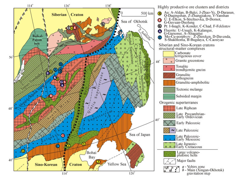
An analysis of geological-geophysical, metallogenic, geochronological, and seismic tomographic studies in territories joining Southeast Russia, East Mongolia, and Northeast China led to the conclusion that deep geodynamics significantly influenced the formation of highly productive ore-magmatic systems in the Late Jurassic-Early Cretaceous. This influence was likely manifested through the initiation of decompression processes around stagnant slab boundaries in the Late Mesozoic. Decompression and advection, which are particularly active near the natural boundaries of the slab, act as triggers for the intense interaction of under and over subduction asthenospheric fluids with adjacent sections of the mantle and for the directed upwelling of powerful flows of matter and energy into the lithosphere. These flows determine the locations of intermediate and peripheral magma chambers: Primary chambers in the lower lithosphere among the metasomatized mantle and lower crust and associated chambers in the middle and upper cratonized parts of the lithosphere. Large ore clusters containing noble metals (Au, PGE), uranium, fluorite, and Cu-Mo-porphyry deposits are associated with late- and postmagmatic derivatives of the emerging magma chambers over the frontal and peripheral (paleotransform) boundaries of a stagnant Pacific slab. These large Late Mesozoic ore clusters and districts form a distinctive "necklace" of strategic materials in East Asia.
Citation: Natalia Boriskina. A «necklace» of large clusters of strategic raw materials over a stagnant oceanic slab in East Asia[J]. AIMS Geosciences, 2024, 10(4): 864-881. doi: 10.3934/geosci.2024040
An analysis of geological-geophysical, metallogenic, geochronological, and seismic tomographic studies in territories joining Southeast Russia, East Mongolia, and Northeast China led to the conclusion that deep geodynamics significantly influenced the formation of highly productive ore-magmatic systems in the Late Jurassic-Early Cretaceous. This influence was likely manifested through the initiation of decompression processes around stagnant slab boundaries in the Late Mesozoic. Decompression and advection, which are particularly active near the natural boundaries of the slab, act as triggers for the intense interaction of under and over subduction asthenospheric fluids with adjacent sections of the mantle and for the directed upwelling of powerful flows of matter and energy into the lithosphere. These flows determine the locations of intermediate and peripheral magma chambers: Primary chambers in the lower lithosphere among the metasomatized mantle and lower crust and associated chambers in the middle and upper cratonized parts of the lithosphere. Large ore clusters containing noble metals (Au, PGE), uranium, fluorite, and Cu-Mo-porphyry deposits are associated with late- and postmagmatic derivatives of the emerging magma chambers over the frontal and peripheral (paleotransform) boundaries of a stagnant Pacific slab. These large Late Mesozoic ore clusters and districts form a distinctive "necklace" of strategic materials in East Asia.

| [1] |
Khomich VG, Boriskina NG (2013) The deep geodynamics of Southeast Russia and the setting of platinum-bearing basite-hyperbasite massifs. J Volcanolog Seismol 7: 328–337. http://dx.doi.org/10.1134/S0742046313040040 doi: 10.1134/S0742046313040040

|
| [2] |
Khomich VG, Boriskina NG (2014) Deep geodynamics and uranium giants of Southeastern Russia. Dokl Earth Sci 458: 1226–1229. http://dx.doi.org/10.1134/S1028334X14100249 doi: 10.1134/S1028334X14100249
|
| [3] |
Khomich VG, Boriskina NG, Santosh M (2018) Super large mineral deposits and deep mantle dynamics: The scenario from Southeast Trans-Baikal region, Russia. Geol J 53: 412–423. https://doi.org/10.1002/gj.2908 doi: 10.1002/gj.2908
|
| [4] |
Khomich VG, Boriskina NG, Santosh M (2014) A geodynamic perspective of world-class gold deposits in East Asia. Gondwana Res 26: 816–833. https://doi.org/10.1016/j.gr.2014.05.007 doi: 10.1016/j.gr.2014.05.007
|
| [5] |
Khomich VG, Boriskina NG, Santosh M (2015) Geodynamics of Late Mesozoic PGE, Au, and U mineralization in the Aldan shield, North Asian Craton. Ore Geol Rev 68: 30–42. http://dx.doi.org/10.1016/j.oregeorev.2015.01.007 doi: 10.1016/j.oregeorev.2015.01.007
|
| [6] |
Khomich VG, Boriskina NG (2019) Paleovolcanic necks and extrusions: Indicators of large uranium orebelts in the territories joining Russia, Mongolia, and China. J Volcanol Geotherm Res 383: 88–102. https://doi.org/10.1016/j.jvolgeores.2018.05.004 doi: 10.1016/j.jvolgeores.2018.05.004
|
| [7] | Seminskiy ZV (2021) Clusters of mineral deposits of the Southern East Siberia and prospects for their development: an overview of the problem. Geodyn Tectonophysics 12: 754–768. |
| [8] | Zonenshain LP, Kuzmin MI, Natapov LM (1990) Tectonics of lithosphere plates of the USSR territory: in 2 books, Moscow: Nedra. Available from: https://www.geokniga.org/books/6515 |
| [9] | Parfenov LM, Berzin NA, Khanchuk AI, et al. (2003) Model of formation of orogenic belts of Central and North-East Asia. Tikhookeanskaya Geologiya 22: 7–41. |
| [10] | Shatkov GA, Volsky AS (2004) Tectonics, deep structure, and minerageny of the Amur river region and neighboring areas. St. Petersburg: VSEGEI. |
| [11] | Gordienko IV (2014) Metallogeny of various geodynamic settings of the Mongolia-Transbaikalia region. Geol Miner Resour Sib S3–1: 7–13. |
| [12] |
Yarmolyuk VV, Kudryashov EA, Kozlovsky AM, et al. (2011) Late Cenozoic volcanic province in Central and East Asia. Petrology 19: 327–347. http://dx.doi.org/10.1134/S0869591111040072 doi: 10.1134/S0869591111040072
|
| [13] | Didenko AI, Malyshev YuF, Saksin BG (2010) Deep structure and metallogeny of East Asia, Vladivostok: Dalnauka. Available from: https://search.rsl.ru/ru/record/01004906622?ysclid = m2mxy27n73631732383. |
| [14] |
Didenko AN, Nosyrev MY, Gil'manova GZ (2022) A gravity-derived Moho model for the Sikhote Alin orogenic belt. Pure Appl Geophys 179: 3967–3988. https://doi.org/10.1007/s00024-021-02842-8 doi: 10.1007/s00024-021-02842-8
|
| [15] | Grachev AF (1996) The main problems of the latest tectonics and geodynamics of Northern Eurasia. Izv Phys Solid Earth 12: 5–36. |
| [16] |
Larin AM (2014) Ulkan-Dzhugdzhur ore-bearing anorthosite-rapakivi granite-peralkaline granite association, Siberian Craton: Age, tectonic setting, sources, and metallogeny. Geol Ore Deposits 56: 257–280. https://doi.org/10.1134/S1075701514040047 doi: 10.1134/S1075701514040047
|
| [17] |
Larin AM, Kotov AB, Salnikova EB, et al. (2023) Age and tectonic setting of the kopri-type granitoids at the Junction Zone of the Dzhugdzhur-Stanovoi and Western Stanovoi superterranes of the Central Asian fold belt. Dokl Earth Sc 509: 111–117. https://doi.org/10.1134/S1028334X22601821 doi: 10.1134/S1028334X22601821
|
| [18] |
Sorokin AA, Sorokin AP, Ponomorchuk VA, et al. (2009) Late Mesozoic volcanism of the eastern part of the Argun superterrane (Far East): Geochemistry and 40Ar/39Ar geochronology. Stratigr Geol Correl 17: 645–658. https://doi.org/10.1134/S0869593809060069 doi: 10.1134/S0869593809060069
|
| [19] |
Li XC, Fan HR, Santosh M, et al. (2012) An evolving magma chamber within extending lithosphere: An integrated geochemical, isotopic and zircon U–Pb geochronological study of the Gushan granite, eastern North China Craton. J Asian Earth Sci 50: 27–43. https://doi.org/10.1016/j.jseaes.2012.01.016 doi: 10.1016/j.jseaes.2012.01.016
|
| [20] |
Ouyang HG, Mao JW, Zhou ZH, et al. (2015) Late Mesozoic metallogeny and intracontinental magmatism, southern Great Xing'an Range, northeastern China. Gondwana Res 27: 1153–1172. http://dx.doi.org/10.1016/j.gr.2014.08.010 doi: 10.1016/j.gr.2014.08.010
|
| [21] |
Zhou JB, Wilde SA, (2013) The crustal accretion history and tectonic evolution of the NE China segment of the Central Asian Orogenic Belt. Gondwana Res 23: 1365–1377. http://dx.doi.org/10.1016/j.gr.2012.05.012 doi: 10.1016/j.gr.2012.05.012
|
| [22] |
Zhao R, Wang QF, Liu XF, et al. (2016) Architecture of the Sulu crustal suture between the North China Craton and Yangtze Craton: Constraints from Mesozoic granitoids. Lithos 266–267: 348–361. http://dx.doi.org/10.1016/j.lithos.2016.10.018 doi: 10.1016/j.lithos.2016.10.018
|
| [23] |
Larin AM, Kotov AB, Salnikova EB, et al. (2021) Age and tectonic setting of granitoids of the Uda Complex of the Dzhugdzhur block of the Stanovoy suture: new data on the formation of giant magmatic belts in Eastern Asia. Dokl Earth Sci 498: 362–366 https://doi.org/10.1134/S1028334X21050081 doi: 10.1134/S1028334X21050081
|
| [24] |
Fan WM, Guo F, Wang YJ, et al. (2003) Late Mesozoic calc-alkaline volcanism of post-orogenic extension in the northern Da Hinggan Mountains, northeastern China. J Volcanol Geotherm Res 121: 115–135. https://doi.org/10.1016/S0377-0273(02)00415-8 doi: 10.1016/S0377-0273(02)00415-8
|
| [25] |
Fan HR, Hu FF, Yang JH, et al. (2007) Fluid evolution and large-scale gold metallogeny during Mesozoic tectonic transition in the Jiaodong Peninsula, eastern China. Geol Soc London Spec Publ 280: 303–316. https://doi.org/10.1144/SP280.16 doi: 10.1144/SP280.16
|
| [26] |
Gordienko IV (2001) Geodynamic evolution of the Central-Asian and Mongol-Okhotsk fold belts and formation of the endogenic deposits. Geosci J 5: 233–241. https://doi.org/10.1007/BF02910306 doi: 10.1007/BF02910306
|
| [27] |
Sun JG, Han SJ, Zhang Y, et al. (2013) Diagenesis and metallogenetic mechanisms of the Tuanjiegou gold deposit from the Lesser Xing'an Range, NE China: Zircon U-Pb geochronology and Lu-Hf isotopic constraints. J Asian Earth Sci 62: 373–388. https://doi.org/10.1016/j.jseaes.2012.10.021 doi: 10.1016/j.jseaes.2012.10.021
|
| [28] |
Ren YS, Chen C, Zou XT, et al. (2016) The age, geological setting, and types of gold deposits in the Yanbian and adjacent areas, NE China. Ore Geol Rev 73: 284–297. https://doi.org/10.1016/j.oregeorev.2015.03.013 doi: 10.1016/j.oregeorev.2015.03.013
|
| [29] |
Chen YJ, Zhang C, Wang P, et al. (2017) The Mo deposits of Northeast China: A powerful indicator of tectonic settings and associated evolutionary trends. Ore Geol Rev 81: 602–640. http://dx.doi.org/10.1016/j.oregeorev.2016.04.017 doi: 10.1016/j.oregeorev.2016.04.017
|
| [30] |
Li Q, Santosh M, Li SR, et al. (2015) Petrology, geochemistry and zircon U–Pb and Lu–Hf isotopes of the Cretaceous dykes in the central North China Craton: Implications for magma genesis and gold metallogeny. Ore Geol Rev 67: 57–77. https://doi.org/10.1016/j.oregeorev.2014.11.015 doi: 10.1016/j.oregeorev.2014.11.015
|
| [31] |
Andreeva OV, Petrov VA, Poluektov VV (2020) Mesozoic acid magmatites of Southeastern Transbaikalia: petrogeochemistry and relationship with metasomatism and ore formation. Geol Ore Deposits 62: 69–96. https://doi.org/10.1134/S1075701520010018 doi: 10.1134/S1075701520010018
|
| [32] |
Zhao D, Pirajno F, Dobretsov NL, et al. (2010) Mantle structure and dynamics under East Russia and adjacent regions. Russ Geol Geophys 51: 925–938. https://doi.org/10.1016/j.rgg.2010.08.003 doi: 10.1016/j.rgg.2010.08.003
|
| [33] |
Deng J, Wang Q (2016) Gold mineralization in China: Metallogenic provinces, deposit types and tectonic framework. Gondwana Res 36: 219–274. https://doi.org/10.1016/j.gr.2015.10.003 doi: 10.1016/j.gr.2015.10.003
|
| [34] |
Zonenshain LP, Savostin LA (1981) Geodynamics of the Baikal Rift System and Plate Tectonics of Asia. Tectonophysics 76: 1–45. https://doi.org/10.1016/0040-1951(81)90251-1 doi: 10.1016/0040-1951(81)90251-1
|
| [35] |
Kepezhinskas PK, Kepezhinskas NP, Berdnikov NV, et al. (2020) Native metals and intermetallic compounds in subduction-related ultramafic rocks from the Stanovoy mobile belt (Russian Far East): implications for redox heterogeneity in subduction zones. Ore Geol Rev 127: 103800. https://doi.org/10.1016/j.oregeorev.2020.103800 doi: 10.1016/j.oregeorev.2020.103800
|
| [36] |
Kepezhinskas P, Berdnikov N, Kepezhinskas N, et al. (2022) Adakites, high-Nb basalts and copper-gold depositions in magmatic arcs and collictional orogens: an overview. Geosciences 12: 29. https://doi.org/10.3390/geosciences12010029 doi: 10.3390/geosciences12010029
|
| [37] |
Malyshev YF, Podgornyi VY, Shevchenko BF, et al. (2007) Deep structure of the Amur lithospheric plate border zone. Russ J Pac Geol 1: 107–119. https://doi.org/10.1134/S1819714007020017 doi: 10.1134/S1819714007020017
|
| [38] |
Maruyama S, Santosh M, Zhao D (2007) Superplume, supercontinent, and post-perovskite: Mantle dynamics and antiplate tectonics on the Core-Mantle Boundary. Gondwana Res 11: 7–37. http://dx.doi.org/10.1016/j.gr.2006.06.003 doi: 10.1016/j.gr.2006.06.003
|
| [39] | Li C, van der Hilst RD (2010) Structure of the upper mantle and transition zone beneath Southeast Asia from traveltime tomography. J Geophys Res Solid Earth 115: B07308. https://doi.org/10.1029/2009JB006882 |
| [40] |
Li J, Wang X, Wang X, et al. (2013) P and SH velocity structure in the upper mantle beneath Northeast China: Evidence for a stagnant slab in hydrous mantle transition zone. Earth Planet Sci Lett 367: 71–81. https://doi.org/10.1016/j.epsl.2013.02.026 doi: 10.1016/j.epsl.2013.02.026
|
| [41] | Zhao D, Tian Y (2013) Changbai intraplate volcanism and deep earthquakes in East Asia: a possible link? Geophys J Int 195: 706–724. |
| [42] |
Jiang G, Zhang G, Zhao D, et al. (2015) Mantle dynamics and cretaceous magmatism in east-central China: Insight from teleseismic tomograms. Tectonophysics 664: 256–268. http://dx.doi.org/10.1016/j.tecto.2015.09.019 doi: 10.1016/j.tecto.2015.09.019
|
| [43] |
Khomich VG, Boriskina NG, Kasatkin SA (2019) Geology, magmatism, metallogeny, and geodynamics of the South Kuril Islands. Ore Geol Rev 105: 151–162. https://doi.org/10.1016/j.oregeorev.2018.12.015 doi: 10.1016/j.oregeorev.2018.12.015
|
| [44] |
Khomich VG, Boriskina NG, Santosh M (2016) Geodynamic framework of large unique uranium orebelts in Southeast Russia and East Mongolia. J Asian Earth Sci 119: 145–166. http://dx.doi.org/10.1016/j.jseaes.2016.01.018 doi: 10.1016/j.jseaes.2016.01.018
|
| [45] |
Khutorskoi MD, Polyak BG (2017) Special features of heat flow in transform faults of the North Atlantic and Southeast Pacific. Geotectonics 51: 152–162. https://doi.org/10.1134/S0016852117010022 doi: 10.1134/S0016852117010022
|
| [46] |
Goldfarb RJ, Santosh M (2014) The dilemma of the Jiaodong gold deposits: are they unique? Geosci Front 5: 139–153. http://dx.doi.org/10.1016/j.gsf.2013.11.001 doi: 10.1016/j.gsf.2013.11.001
|
| [47] |
Mao XC, Ren J, Liu ZK, et al. (2019) Three-dimensional prospectivity modeling of the Jiaojia-type gold deposit, Jiaodong Peninsula, Eastern China: A case study of the Dayingezhuang deposit. J Geochem Explor 203: 27–44. https://doi.org/10.1016/j.gexplo.2019.04.002 doi: 10.1016/j.gexplo.2019.04.002
|
| [48] |
Chen Y, Guo G, Li X (1998) Metallogenic geodynamic background of Mesozoic gold deposits in granite-greenstone terrains of North China Craton. Sci China Ser D-Earth Sci 41: 113–120. https://doi.org/10.1007/BF02932429 doi: 10.1007/BF02932429
|
| [49] | Zorin YA, Turutanov EK, Kozhevnikov VM, et al. (2006) On the nature of Cenozoic upper mantle plumes in Eastern Siberia (Russia) and Central Mongolia. Russ Geol Geophys 47: 1056–1070. |
| [50] |
Khomich VG, Boriskina NG (2009) Relationship between the gold bearing areas and gradient sones of the gravity field of southeastern regions of Russia. Dokl Earth Sc 428: 1100–1104. http://dx.doi.org/10.1134/S1028334X09070137 doi: 10.1134/S1028334X09070137
|
| [51] | Laverov NP, Velichkin VI, Vlasov BP, et al. (2012) Uranium and molybdenum-uranium deposits in the areas of continental intracrustal magmatism: geology, geodynamic and physico-chemical conditions of formation. Moscow: IFSN RAN IGEM RAN. |
| [52] |
Berzina AP, Berzina AN, Gimon VO, et al. (2015) The Zhireken porphyry Mo ore-magmatic system (Eastern Transbaikalia): U-Pb age, sources, and geodynamic setting. Russ Geol Geophys 56: 446–465. https://doi.org/10.1016/j.rgg.2015.02.006 doi: 10.1016/j.rgg.2015.02.006
|
| [53] | Mashkovtsev GA, Korotkov VV, Rudnev VV (2020) Ore-bearing of the Mesozoic tectonic-magmatic activation area of the Eastern Siberia and the Far East. Prospect Prot Miner Resour 11: 5–7. |
| [54] | Vetluzhskikh VG, Kazansky VI, Kochetkov AY, et al. (2002) Central Aldan gold deposits. Geol Ore Deposits 44: 405–434. Available from: https://www.pleiades.online/cgi-perl/search.pl?type = abstract & name = geolore & number = 6 & year = 2 & page = 405. |
| [55] | Shatov VV, Molchanov AV, Shatova NV, et al. (2012) Petrography, geochemistry and isotopic (U-Pb and Rb-Sr) dating of alkaline magmatic rocks of the Ryabinovy massif (South Yakutia). Reg Geol Metallog 51: 62–78. |
| [56] |
Chernyshev IV, Prokof'ev VY, Bortnikov NS, et al. (2014) Age of granodiorite porphyry and beresite from the Darasun gold field, Eastern Transbaikal region, Russia. Geol Ore Deposits 56: 1–14. https://doi.org/10.1134/S1075701514010036 doi: 10.1134/S1075701514010036
|
| [57] | Andreeva OV, Golovin VA, Kozlova PS, et al. (1996) Evolution of mesozoic magmatism and ore-forming metasomatic processes in the Southeastern Transbaikal region (Russia). Geol Ore Deposits 38: 101–113. |
| [58] |
Stupak FM, Kudryashova EA, Lebedev VA, et al. (2018) The structure, composition, and conditions of generation for the early cretaceous Mongolia—East-Transbaikalia volcanic belt: the Durulgui–Torei area (Southern Transbaikalia, Russia). J Volcanolog Seismol 12: 34–46. https://doi.org/10.1134/S0742046318010074 doi: 10.1134/S0742046318010074
|
| [59] |
Ponomarchuk AV, Prokopyev IR, Svetlitskaya TV, et al. (2019) 40Ar/39Ar geochronology of alkaline rocks of the Inagli massif (Aldan Shield, Southern Yakutia). Russ Geol Geophys 60: 33–44. https://doi.org/10.15372/RGG2019003 doi: 10.15372/RGG2019003
|
| [60] |
Gaskov IV, Borisenko AS, Borisenko ID, et al. (2023) Chronology of alkaline magmatism and gold mineralization in the Central Aldan ore district (Southern Yakutia). Russ Geol Geophys 64: 175–191. https://doi.org/10.2113/RGG20214427 doi: 10.2113/RGG20214427
|
| [61] |
Shukolyukov YA, Yakubovich OV, Mochalov AG, et al. (2012) New geochronometer for the direct isotopic dating of native platinum minerals (190Pt-4He method). Petrology 20: 491–505. http://dx.doi.org/10.1134/S0869591112060033 doi: 10.1134/S0869591112060033
|
| [62] |
Ronkin YL, Efimov AA, Lepikhina GA, et al. (2013) U-Pb dating of the baddeleytte-zircon system from Pt-bearing dunite of the Konder massif, Aldan Shield: New data. Dokl Earth Sc 450: 607–612. https://doi.org/10.1134/S1028334X13060135 doi: 10.1134/S1028334X13060135
|
| [63] |
Mochalov AG, Yakubovich OV, Bortnikov NS (2016) 190Pt–4He age of PGE ores in the alkaline–ultramafic Konder massif (Khabarovsk district, Russia). Dokl Earth Sc 469: 846–850. https://doi.org/10.1134/S1028334X16080134 doi: 10.1134/S1028334X16080134
|
| [64] |
Mochalov AG, Yakubovich OV, Bortnikov NS (2022) 190Pt–4He dating of placer-forming minerals of platinum from the Chad alkaline-ultramafic massif: new evidence of the polycyclic nature of ore formation. Dokl Earth Sc 504: 240–247. https://doi.org/10.1134/S1028334X22050105 doi: 10.1134/S1028334X22050105
|
| [65] | Kazansky VI (2004) The unique Central Aldan gold-uranium ore district (Russia). Geol Ore Deposits 46: 167–181. |
| [66] | Mashkovtsev GA, Konstantinov AK, Miguta AK, et al. (2010) Uranium of Russian entrails, Moscow: VIMS. Available from: https://elib.biblioatom.ru/text/uran-rossiyskih-nedr_2010/p0/. |
| [67] | Afanasyev GV, Mironov YB, Pinsky EM (2018) Role of combined paleohydrogeological systems in forming uranium mineralization in volcano-tectonic depressions of the Central Asian mobile belt. Reg Geol Metallog 3: 77–87. |
| [68] | Rui GZ (2010) Discussion on the geological characteristics and origin of the 460 large uranium-molybdenum deposit. World Nucl Geol 27: 149–154. |
| [69] | Wu JH, Ding H, Niu ZL, et al. (2015) SHRIMP zircon U-Pb dating of country rock in Zhangmajing U-Mo deposit in Guyuan, Hebei Province, and its geological significance. Mineral Deposit 4: 757–768. |
| [70] |
Wang JQ, Liu GJ, Dong S, et al. (2023) The "trinity" prospecting prediction geological model of the Zhangmajing uranium molybdenum deposit in Guyuan County, Hebei Province. Geol Bull China 42: 931–940. http://dx.doi.org/10.12097/j.issn.1671-2552.2023.06.006 doi: 10.12097/j.issn.1671-2552.2023.06.006
|
| [71] | Rybalov BL (2000) Evolutionary rows of Late Mesozoic ore deposits of the Eastern Transbaikal region (Russia). Geol Ore Deposits 42: 340–350. |
| [72] |
Berzina AP, Berzina AN, Gimon VO (2014) Geochemical and Sr–Pb–Nd isotopic characteristics of the Shakhtama porphyry Mo-Cu system (Eastern Transbaikalia, Russia). J Asian Earth Sci 79: 655–665. http://dx.doi.org/10.1016/j.jseaes.2013.07.028 doi: 10.1016/j.jseaes.2013.07.028
|
| [73] |
Berzina AP, Berzina AN, Gimon VO (2016) Paleozoic-Mesozoic porphyry Cu (Mo) and Mo (Cu) deposits within the southern margin of the Siberian Craton: geochemistry, geochronology, and petrogenesis (a Review). Minerals 6: 125. http://dx.doi.org/10.3390/min6040125 doi: 10.3390/min6040125
|
| [74] | Pushkarev YD, Kostoyanov AI, Orlova MP, et al. (2002) Features of Rb-Sr, Sm-Nd, Pb-Pb, Re-Os and K-Ar isotope systems in the Konder massif: mantle substrate enriched in platinum group metals. Reg Geol Metallog 16: 80–91. |
| [75] |
Simonov VA, Prikhodko VS, Kovyazin SV (2011) Genesis of platiniferous massifs in the Southeastern Siberian platform. Petrology 19: 549–567. http://dx.doi.org/10.1134/S0869591111050043 doi: 10.1134/S0869591111050043
|
| [76] |
Shatkov GA, Antonov AV, Butakov PM, et al. (2014) Uranyl molybdates in fluorites and uranium-carbonate ores from the Streltsovskoe ore field of the Argun deposit. Dokl Earth Sc 456: 764–768. https://doi.org/10.1134/S1028334X14060373 doi: 10.1134/S1028334X14060373
|
| [77] | Konstantinov MM, Politov VK, Novikov VP, et al. (2002) Geological structure of gold districts of volcano-plutonic belts in Eastern Russia. Geol Ore Deposits 44: 252–266. |
| [78] |
Dobretsov NL, Koulakov I, Kukarina EV, et al. (2015) An integrate model of subduction: contributions from geology, experimental petrology, and seismic tomography. Russ Geol Geophys 56: 13–38. https://doi.org/10.1016/j.rgg.2015.01.002 doi: 10.1016/j.rgg.2015.01.002
|
| [79] | Pechenkin IG (2016) Relationship between uranium metallogeny and geodynamic processes in the marginal parts of Eurasia. Ores Metals 2: 5–17. |


Figures(5) / Tables(1)

Natalia Boriskina. A «necklace» of large clusters of strategic raw materials over a stagnant oceanic slab in East Asia[J]. AIMS Geosciences, 2024, 10(4): 864-881. doi: 10.3934/geosci.2024040


 DownLoad: