


Figure 1.
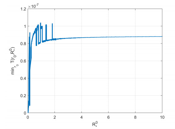
The graph of with .
With the continuous development of Internet of Things, finance, big data and many other fields, blockchain has been widely used in these areas for transactions, data sharing, product traceability and so on. Numerous assets have appeared in the blockchain, and there are some levels of conflicts among privacy protection of these assets, transaction transparency and auditability in blockchain; so how to provide privacy preserving, make public verifications and audit the encrypted assets are challenging problems. In this paper, we propose a privacy-preserving transaction scheme with public verification and reliable audit in blockchain. First, we provide privacy preserving of transaction contents based on homomorphic encryption. It is flexible, as we decouple user identity and transaction contents. Then, we propose and design a multiplicative zero-knowledge proof with formal security analysis. Furthermore, several verification rules are defined by us in the scheme, such as balance verification and multiplicative verification based on the proposed multiplicative zero-knowledge proof. Our scheme enables reliable and offline auditing for each transaction, and we aggregate the zero-knowledge proofs to save the ledger space. Finally, we make a security analysis of our proposal in terms of transaction confidentiality, public verification and audit reliability, and we give a performance analysis of the proposed scheme.
Citation: Shuang Yao, Dawei Zhang. A blockchain-based privacy-preserving transaction scheme with public verification and reliable audit[J]. Electronic Research Archive, 2023, 31(2): 729-753. doi: 10.3934/era.2023036
| [1] | Shihe Xu, Junde Wu . Qualitative analysis of a time-delayed free boundary problem for tumor growth with angiogenesis and Gibbs-Thomson relation. Mathematical Biosciences and Engineering, 2019, 16(6): 7433-7446. doi: 10.3934/mbe.2019372 |
| [2] | H. J. Alsakaji, F. A. Rihan, K. Udhayakumar, F. El Ktaibi . Stochastic tumor-immune interaction model with external treatments and time delays: An optimal control problem. Mathematical Biosciences and Engineering, 2023, 20(11): 19270-19299. doi: 10.3934/mbe.2023852 |
| [3] | Yuting Ding, Gaoyang Liu, Yong An . Stability and bifurcation analysis of a tumor-immune system with two delays and diffusion. Mathematical Biosciences and Engineering, 2022, 19(2): 1154-1173. doi: 10.3934/mbe.2022053 |
| [4] | Alessandro Bertuzzi, Antonio Fasano, Alberto Gandolfi, Carmela Sinisgalli . Interstitial Pressure And Fluid Motion In Tumor Cords. Mathematical Biosciences and Engineering, 2005, 2(3): 445-460. doi: 10.3934/mbe.2005.2.445 |
| [5] | Jiaxin Nan, Wanbiao Ma . Stability and persistence analysis of a microorganism flocculation model with infinite delay. Mathematical Biosciences and Engineering, 2023, 20(6): 10815-10827. doi: 10.3934/mbe.2023480 |
| [6] | Maria Vittoria Barbarossa, Christina Kuttler, Jonathan Zinsl . Delay equations modeling the effects of phase-specific drugs and immunotherapy on proliferating tumor cells. Mathematical Biosciences and Engineering, 2012, 9(2): 241-257. doi: 10.3934/mbe.2012.9.241 |
| [7] | Marek Bodnar, Monika Joanna Piotrowska, Urszula Foryś . Gompertz model with delays and treatment: Mathematical analysis. Mathematical Biosciences and Engineering, 2013, 10(3): 551-563. doi: 10.3934/mbe.2013.10.551 |
| [8] | Qiaoling Chen, Fengquan Li, Sanyi Tang, Feng Wang . Free boundary problem for a nonlocal time-periodic diffusive competition model. Mathematical Biosciences and Engineering, 2023, 20(9): 16471-16505. doi: 10.3934/mbe.2023735 |
| [9] | Avner Friedman, Harsh Vardhan Jain . A partial differential equation model of metastasized prostatic cancer. Mathematical Biosciences and Engineering, 2013, 10(3): 591-608. doi: 10.3934/mbe.2013.10.591 |
| [10] | Hui Cao, Dongxue Yan, Ao Li . Dynamic analysis of the recurrent epidemic model. Mathematical Biosciences and Engineering, 2019, 16(5): 5972-5990. doi: 10.3934/mbe.2019299 |
With the continuous development of Internet of Things, finance, big data and many other fields, blockchain has been widely used in these areas for transactions, data sharing, product traceability and so on. Numerous assets have appeared in the blockchain, and there are some levels of conflicts among privacy protection of these assets, transaction transparency and auditability in blockchain; so how to provide privacy preserving, make public verifications and audit the encrypted assets are challenging problems. In this paper, we propose a privacy-preserving transaction scheme with public verification and reliable audit in blockchain. First, we provide privacy preserving of transaction contents based on homomorphic encryption. It is flexible, as we decouple user identity and transaction contents. Then, we propose and design a multiplicative zero-knowledge proof with formal security analysis. Furthermore, several verification rules are defined by us in the scheme, such as balance verification and multiplicative verification based on the proposed multiplicative zero-knowledge proof. Our scheme enables reliable and offline auditing for each transaction, and we aggregate the zero-knowledge proofs to save the ledger space. Finally, we make a security analysis of our proposal in terms of transaction confidentiality, public verification and audit reliability, and we give a performance analysis of the proposed scheme.
Over the past few decades, considerable attention has been paid to the rigorous analysis of mathematical models describing tumor growth and great progress has been achieved. Most work in this direction focuses on the sphere-shaped or nearly sphere-shaped tumor models; see [1,2,3,4,5,6,7,8,9] and the references therein. Observing that the work concerning models for tumors having different geometric configurations from spheroids is less frequent, in this paper we are interested in the situation of tumor cord–a kind of tumor that grows cylindrically around the central blood vessel and receives nutrient materials (such as glucose and oxygen) from the blood vessel [10]. The model only describes the evolution of the tumor cord section perpendicular to the length direction of the blood vessel due to the cord's uniformity in that direction. Assume that the radius of the blood vessel is r0 and denote by J and Γ(t) the section of the blood vessel wall and the section of the exterior surface of the tumor cord, respectively, then J={x∈R2;|x|=r0}. We also denote by Ω(t) the region of the section of the tumor cord, so that Ω(t) is an annular-like bounded domain in R2 and ∂Ω(t)=J∪Γ(t). The mathematical formulation of the tumor model under study is as follows:
| cσt(x,t)−Δσ(x,t)+σ(x,t)=0,x∈Ω(t),t>0, | (1.1) |
| −Δp(x,t)=μ[σ(ξ(t−τ;x,t),t−τ)−˜σ],x∈Ω(t),t>0, | (1.2) |
| {dξds=−∇p(ξ,s),t−τ≤s≤t,ξ=x,s=t, | (1.3) |
| σ(x,t)=ˉσ,∂→np(x,t)=0,x∈J,t>0, | (1.4) |
| ∂→νσ(x,t)=0,p(x,t)=γκ(x,t),x∈Γ(t),t>0, | (1.5) |
| V(x,t)=−∂→νp(x,t),x∈Γ(t),t>0, | (1.6) |
| Γ(t)=Γ0,−τ≤t≤0, | (1.7) |
| σ(x,t)=σ0(x),x∈Ω0,−τ≤t≤0, | (1.8) |
| p(x,t)=p0(x),x∈Ω0,−τ≤t≤0. | (1.9) |
Here, σ and p denote the nutrient concentration and pressure within the tumor, respectively, which are to be determined together with Ω(t), and c=Tdiffusion /Tgrowth is the ratio of the nutrient diffusion time scale to the tumor growth (e.g., tumor doubling) time scale; thus, it is very small and can sometimes be set to be 0 (quasi-steady state approximation). Assume that the time delay τ is reflected between the time at which a cell commences mitosis and the time at which the daughter cells are produced and ξ(s;x,t) represents the cell location at time s as cells are moving with the velocity field →V, then the function ξ(s;x,t) satisfies
| {dξds=→V(ξ,s),t−τ≤s≤t,ξ|s=t=x. | (1.10) |
In other words, ξ tracks the path of the cell currently located at x. (1.3) is further derived from (1.10) under the assumption of a porous medium structure for the tumor, where Darcy's law →V=−∇p holds true. Because of the presence of time delay, the tumor grows at a rate that is related to the nutrient concentration when it starts mitosis and a combination of the conservation of mass and Darcy's law yields (1.2), in which μ represents the growth intensity of the tumor and ˜σ is the nutrient concentration threshold required for tumor cell growth. Additionally, ˉσ is the nutrient concentration in the blood vessel, ˉσ>˜σ, V, κ and →ν denote the normal velocity, the mean curvature and the unit outward normal field of the outer boundary Γ(t), respectively, →n denotes the unit outward normal field of the fixed inner boundary J, and γ is the outer surface tension coefficient. Thus, the boundary condition σ=ˉσ on J indicates that the tumor receives constant nutrient supply from the blood vessel, ∂→νσ=0 on Γ(t) implies that the nutrient cannot pass through Γ(t), ∂→np=0 on J means that tumor cells cannot pass through the blood vessel wall, p=γκ on Γ(t) is due to the cell-to-cell adhesiveness, and V=−∂→νp on Γ(t) is the well-known Stefan condition representing that the normal velocity of the tumor cord outer boundary Γ(t) is the same with that of tumor cells adjacent to Γ(t). Finally, σ0(x), p0(x), Γ0 are given initial data and Ω(t)=Ω0 for −τ≤t≤0.
Before going to our interest, we prefer to recall some relevant works. Models for the growth of the strictly cylindrical tumor cord were studied in [11,12,13]. For the model (1.1)–(1.9) without the time delay, if c=0, Zhou and Cui [14] showed that the unique radially symmetric stationary solution exists and is asymptotically stable for any sufficiently small perturbations. Meanwhile, if c>0, Wu et al. [15] proved that the stationary solution is locally asymptotically stable provided that c is small enough. On the other hand, Zhao and Hu [16] considered the multicell spheroids with time delays. For the case c=0, they analyzed the linear stability of the radially symmetric stationary solution as well as the impact of the time delay.
Motivated by the works [14,15,16], here we aim to discuss the linear stability of stationary solutions to the problem (1.1)–(1.9) with the quasi-steady-state assumption, i.e., c=0, and investigate the effect of time delay on tumor growth. Our first main result is given below.
Theorem 1.1. For small time delay τ, the problem (1.1)–(1.9) admits a unique radially symmetric stationary solution.
Next, in order to deal with the linear stability of the radially symmetric stationary solution, denoted by (σ∗,p∗,Ω∗), where Ω∗={x∈R2: r0<r=|x|<R∗}, we assume that the initial conditions are perturbed as follows:
| Ω(t)={x∈R2:r0<r<R∗+ερ0(θ)},−τ≤t≤0,σ(r,θ,t)=σ∗(r)+εw0(r,θ),p(r,θ,t)=p∗(r)+εq0(r,θ),−τ≤t≤0. |
The linearized problem of (1.1)–(1.9) at (σ∗,p∗,Ω∗) is then obtained by substituting
| Ω(t):r0<r<R∗+ερ(θ,t)+O(ε2), | (1.11) |
| σ(r,θ,t)=σ∗(r)+εw(r,θ,t)+O(ε2), | (1.12) |
| p(r,θ,t)=p∗(r)+εq(r,θ,t)+O(ε2) | (1.13) |
into (1.1)–(1.9) and collecting the ε-order terms. Now, we can state the second main result of this paper.
Theorem 1.2. For small time delay τ, the radially symmetric stationary solution (σ∗,p∗,Ω∗) of (1.1)–(1.9) with c=0 is linearly stable, i.e.,
| max0≤θ≤2π|ρ(θ,t)|≤Ce−δt,t>0 | (1.14) |
for some positive constants C and δ.
Remark 1.1. Compared with results of the problem modeling the growth of tumor cord without time delays in [14], the introduction of the time delay does not affect the stability of the radially symmetric stationary solution even under non-radial perturbations. However, as we shall see in Subsection 3.3, the numerical result shows that adding time delay would result in a larger stationary tumor. Moreover, the stronger the growth intensity of the tumor is, the greater the influence of time delay on the size of the stationary tumor is.
Remark 1.2. Compared with results of the nearly sphere-shaped tumor model with time delays in [16], which state that the radially symmetric stationary solution is linearly stable for small μ in the sense that limt→∞max0≤θ≤2π|ρ(θ,t)−(a1cosθ+b1sinθ)|=0 for some constants a1 and b1, the radially symmetric stationary solution of tumor cord with the time delay is linearly stable for any μ>0 in the normal sense.
This paper is organized as follows. In Section 2, we give the proof of Theorem 1.1 by first transforming the free boundary problem into an equivalent problem with fixed boundary and then applying the contraction mapping principle combined with Lp estimates to this fixed boundary problem. In Section 3, we prove Theorem 1.2 and Remark 1.1 by first introducing the linearization of (1.1)–(1.9) at the radially symmetric stationary solution (σ∗,p∗,Ω∗), and then making a delicate analysis of the expansion in the time delay τ provided that τ is sufficiently small. A brief conclusion in Section 4 completes the paper.
In this section, we study radially symmetric stationary solutions (σ∗,p∗,Ω∗) to the system (1.1)–(1.9), which satisfy
| −Δrσ∗(r)+σ∗(r)=0,σ∗(r0)=ˉσ,σ′∗(R∗)=0,r0<r<R∗, | (2.1) |
| −Δrp∗(r)=μ[σ∗(ξ(−τ;r,0))−˜σ],p′∗(r0)=0,p∗(R∗)=γR∗,r0<r<R∗, | (2.2) |
| {dξds(s;r,0)=−∂p∗∂r(ξ(s;r,0)),−τ≤s≤0,ξ(s;r,0)=r,s=0, | (2.3) |
| ∫R∗r0[σ∗(ξ(−τ;r,0))−˜σ]rdr=0, | (2.4) |
where Δr is the radial part of the Laplacian in R2.
Before proceeding further, let us recall that the modified Bessel functions Kn(r) and In(r), standard solutions of the equation
| r2y′′+ry′−(r2+n2)y=0,r>0, | (2.5) |
have the following properties:
| In+1(r)=In−1(r)−2nrIn(r),Kn+1(r)=Kn−1(r)+2nrKn(r),n≥1, | (2.6) |
| I′n(r)=12[In−1(r)+In+1(r)],K′n(r)=−12[Kn−1(r)+Kn+1(r)],n≥1, | (2.7) |
| I′n(r)=In−1(r)−nrIn(r), K′n(r)=−Kn−1(r)−nrKn(r),n≥1, | (2.8) |
| I′n(r)=nrIn(r)+In+1(r), K′n(r)=nrKn(r)−Kn+1(r),n≥0, | (2.9) |
| In(r)Kn+1(r)+In+1(r)Kn(r)=1r,n≥0 | (2.10) |
and
| I′n(r)>0,K′n(r)<0. |
Proof of Theorem 1.1 In view of (2.5), the solution of (2.1) is clearly given by
| σ∗(r)=ˉσI0(r)K1(R∗)+I1(R∗)K0(r)I0(r0)K1(R∗)+I1(R∗)K0(r0). | (2.11) |
Introducing the notations:
| ˆr=r−r0R∗−r0,ˆσ(ˆr)=σ∗(r),ˆp(ˆr)=(R∗−r0)p∗(r),ˆξ(s,ˆr,0)=ξ(s,r,0)−r0R∗−r0, |
(2.1)–(2.4) reduces to the following system after dropping the "^" in the above variables:
| ∂2σ∂r2+R∗−r0r(R∗−r0)+r0∂σ∂r=(R∗−r0)2σ,σ(0)=ˉσ,σ′(1)=0, | (2.12) |
| {∂2p∂r2+R∗−r0r(R∗−r0)+r0∂p∂r=−μ(R∗−r0)3[σ(r+1(R∗−r0)3∫0−τ∂p∂r((R∗−r0)ξ(s;r,0)+r0)ds)−˜σ],p′(0)=0,p(1)=γ(R∗−r0)R∗, | (2.13) |
| {dξds(s;r,0)=−1(R∗−r0)3∂p∂r((R∗−r0)ξ(s;r,0)+r0),−τ≤s≤0,ξ(s;r,0)=r,s=0, | (2.14) |
| ∫10[r(R∗−r0)+r0][σ(r+1(R∗−r0)3∫0−τ∂p∂r((R∗−r0)ξ(s;r,0)+r0)ds)−˜σ]dr=0. | (2.15) |
It is clear that (2.12) can be solved explicitly. For convenience, we extend the solution of (2.12) outside [0, 1]:
| σ(r;R∗)={ˉσI0(r(R∗−r0)+r0)K1(R∗)+I1(R∗)K0(r(R∗−r0)+r0)I0(r0)K1(R∗)+I1(R∗)K0(r0),0≤r≤1,ˉσI0(R∗)K1(R∗)+I1(R∗)K0(R∗)I0(r0)K1(R∗)+I1(R∗)K0(r0),1<r≤2. | (2.16) |
Assume that Rmin and Rmax are positive constants to be determined later and r0<Rmin<Rmax. For any R∗∈[Rmin,Rmax], we will prove that p is also uniquely determined by applying the contraction mapping principle.
Noticing that 0 is a lower solution of (2.14), but there is no assurance that ξ(s;r,0)≤1 for −τ≤s≤0, we suppose ξ(s;r,0)∈[0,2] and take
| X={p∈W2,∞[0,2];‖p‖W2,∞[0,2]≤M}, |
where M>0 is to be determined. For each p∈X, we first solve for ξ from (2.14) and substitute it into (2.13), then the following system
| {∂2ˉp∂r2+R∗−r0r(R∗−r0)+r0∂ˉp∂r=−μ(R∗−r0)3[σ(r+1(R∗−r0)3∫0−τ∂p∂r((R∗−r0)ξ(s;r,0)+r0)ds)−˜σ],ˉp(1)=γ(R∗−r0)R∗,∂ˉp∂r(0)=0 | (2.17) |
allows a unique solution ˉp∈W2,∞[0,1]. Applying the strong maximum principle combined with the Hopf lemma to (2.1) shows that σ(r;R∗)≤ˉσ. Thus, integrating (2.17), we obtain
| ‖1r(R∗−r0)+r0∂ˉp∂r‖L∞[0,1]≤μ2(Rmax−r0)2(ˉσ+˜σ), | (2.18) |
| ‖ˉp‖L∞[0,1]≤γ(Rmax−r0)Rmin+μ4R2max(Rmax−r0)(ˉσ+˜σ), | (2.19) |
| ‖∂2ˉp∂r2‖L∞[0,1]≤3μ2(Rmax−r0)3(ˉσ+˜σ). | (2.20) |
Define the mapping
| Lp(r)={ˉp(r),0≤r≤1,ˉp(1)+ˉp′(1)(r−1),1<r≤2,p∈X, |
then ‖Lp‖∈W2,∞[0,2] and ‖Lp‖W2,∞[0,2]≤2‖ˉp‖W2,∞[0,1]. Combining (2.18)–(2.20), we find
| ‖Lp‖W2,∞[0,2]≤2{μ2(Rmax−r0)2(ˉσ+˜σ)+3μ2(Rmax−r0)3(ˉσ+˜σ)+γ(Rmax−r0)Rmin+μ4R2max(Rmax−r0)(ˉσ+˜σ)}≜M1. | (2.21) |
If we choose M≥M1, then Lp∈X by (2.21) and L maps X to itself.
We now show that L is a contraction. Given p(1),p(2)∈X, one can first get ξ(1),ξ(2) from the following two systems:
| {dξ(1)ds(s;r,0)=−1(R∗−r0)3∂p(1)∂r((R∗−r0)ξ(1)(s;r,0)+r0),−τ≤s≤0,ξ(1)(s;r,0)=r,s=0, | (2.22) |
| {dξ(2)ds(s;r,0)=−1(R∗−r0)3∂p(2)∂r((R∗−r0)ξ(2)(s;r,0)+r0),−τ≤s≤0,ξ(2)(s;r,0)=r,s=0. | (2.23) |
Integrating (2.22) and (2.23) with regard to s over the interval [−τ,0] and making a subtraction yield
| |ξ(1)−ξ(2)|≤τ(R∗−r0)3max−τ≤s≤00≤r≤1[|∂p(1)∂r((R∗−r0)ξ(1)+r0)−∂p(2)∂r((R∗−r0)ξ(1)+r0)|+|∂p(2)∂r((R∗−r0)ξ(1)+r0)−∂p(2)∂r((R∗−r0)ξ(2)+r0)|]≤τ(R∗−r0)3‖p(1)−p(2)‖W2,∞[0,2]+τM(R∗−r0)2max−τ≤s≤00≤r≤1|ξ(1)−ξ(2)| |
for all −τ≤s≤0 and 0≤r≤1. Consequently,
| max−τ≤s≤00≤r≤1|ξ(1)−ξ(2)|≤τ(R∗−r0)3−τM(R∗−r0)‖p(1)−p(2)‖W2,∞[0,2]. | (2.24) |
Next, we substitute ξ(1),ξ(2) into (2.17) and solve for ˉp(1) and ˉp(2), respectively, then it follows from (2.17) that (ˉp(1)−ˉp(2))(1)=0, ∂∂r(ˉp(1)−ˉp(2))(0)=0 and
| −∂2∂r2(ˉp(1)−ˉp(2))−R∗−r0r(R∗−r0)+r0∂∂r(ˉp(1)−ˉp(2))=μ(R∗−r0)3[σ(r+1(R∗−r0)3∫0−τ∂p(1)∂r((R∗−r0)ξ(1)(s;r,0)+r0)ds)−σ(r+1(R∗−r0)3∫0−τ∂p(2)∂r((R∗−r0)ξ(2)(s;r,0)+r0)ds)]. |
Using (2.24), we derive
| ‖1r(R∗−r0)+r0∂∂r(ˉp(1)−ˉp(2))‖L∞[0,1]≤μ2(R∗−r0)2‖σ(r+1(R∗−r0)3∫0−τ∂p(1)∂r((R∗−r0)ξ(1)+r0)ds)−σ(r+1(R∗−r0)3∫0−τ∂p(2)∂r((R∗−r0)ξ(2)+r0)ds)‖L∞[0,1]≤μ2(R∗−r0)‖∂σ∂r‖L∞[0,2]∫0−τ(∂p(1)∂r((R∗−r0)ξ(1)+r0)−∂p(2)∂r((R∗−r0)ξ(2)+r0))ds≤μτ2(R∗−r0)‖∂σ∂r‖L∞[0,2](‖p(1)−p(2)‖W2,∞[0,2]+(R∗−r0)‖p(2)‖W2,∞[0,2]max−τ≤s≤00≤r≤1|ξ(1)−ξ(2)|)≤M2τ‖p(1)−p(2)‖W2,∞[0,2] |
and similarly,
| ‖ˉp(1)−ˉp(2)‖L∞[0,1]≤M3τ‖p(1)−p(2)‖W2,∞[0,2],‖∂2∂r2(ˉp(1)−ˉp(2))‖L∞[0,1]≤M4τ‖p(1)−p(2)‖W2,∞[0,2], |
where
| M2=μˉσRmax2r0(Rmax−r0)3(Rmin−r0)2−Mτ,M3=μˉσR3max4r0(Rmax−r0)2(Rmin−r0)2−Mτ,M4=3μˉσRmax2r0(Rmax−r0)4(Rmin−r0)2−Mτ. |
Here, we employed the fact that
| ‖∂σ∂r‖L∞[0,2]=‖∂σ∂r‖L∞[0,1]≤ˉσRmaxr0(Rmax−r0)2 |
by (2.1) and σ≤ˉσ. Let M5=M2+M3+M4, then M5 is independent of τ and
| ‖ˉp(1)−ˉp(2)‖W2,∞[0,1]≤M5τ‖p(1)−p(2)‖W2,∞[0,2], |
which together with Lp(1)(1)=Lp(2)(1)=γ(R∗−r0)R∗ and (Lp(1))′(0)=(Lp(2))′(0)=0 implies that
| ‖Lp(1)−Lp(2)‖W2,∞[0,2]≤2M5τ‖p(1)−p(2)‖W2,∞[0,2]. |
Hence, if τ is sufficiently small such that 2M5τ<1, then we derive a contracting mapping L. The existence and uniqueness of p are therefore obtained.
It suffices to prove that there exists a unique R∗∈[Rmin,Rmax] satisfying (2.15). Substituting (2.16) into (2.15), we find that it is equivalent to solving the following equation for R:
| G(R,τ)=∫10r(R−r0)+r0R+r0[σ∗(r+1(R−r0)3∫0−τ∂p∗∂r((R−r0)ξ(s;r,0)+r0)ds)−˜σ]dr=0. |
Clearly,
| G(R,0)=∫10(σ∗(r;R)−˜σ)r(R−r0)+r0R+r0dr=∫10σ∗(r;R)r(R−r0)+r0R+r0dr−˜σ2. |
Using Lemma 3.1 and Theorem 3.2 in [14] and the condition ˉσ>˜σ, we know that
| limR→r0G(R,0)=ˉσ−˜σ2>0,limR→∞G(R,0)=−˜σ2<0,∂G(R,0)∂R<0, |
which implies that the equation G(R,0)=0 has a unique solution, denoted by RS, and
| G(12(RS+r0),0)>0,G(32RS,0)<0. |
Since
| ∂G(R,τ)∂R=∂G(R,0)∂R+∂2G(R,η)∂R∂ττ+O(τ2),0≤η≤τ |
when τ is sufficiently small, ∂G(R,τ)∂R and ∂G(R,0)∂R have the same sign. Thus, G(R,τ) is monotone decreasing in R. Using the fact that G(R,τ) is continuous in τ, we further have
| G(12(RS+r0),τ)>0,G(32RS,τ)<0. |
Hence, when τ is sufficiently small, the equation G(R,τ)=0 has a unique solution R∗. Taking Rmin=12(RS+r0) and Rmax=32RS, we complete the proof of the theorem.
This section is devoted to the linear stability of the radially symmetric stationary solution (σ∗,p∗,Ω∗) of the problem (1.1)–(1.9) and the effect of time delay on the stability and the size of the stationary tumor. Let (σ,p,Ω(t)), given by (1.11)–(1.13), be solutions to (1.1)–(1.9), and denote by →er, →eθ the unit normal vectors in r, θ directions, respectively. Written in the rectangular coordinates in R2,
| →er=(cosθ,sinθ)T,→eθ=(−sinθ,cosθ)T. |
Using the notation ξ1(s;r,θ,t), ξ2(s;r,θ,t) for the polar radius and angle of ξ(s;r,θ,t), respectively, we have
| ξ(s;r,θ,t)=ξ1(s;r,θ,t)→er(ξ)=ξ1(s;r,θ,t)(cosξ2(s;r,θ,t),sinξ2(s;r,θ,t))T. |
Expand ξ1, ξ2 in ε as
| {ξ1=ξ10+εξ11+O(ε2),ξ2=ξ20+εξ21+O(ε2), | (3.1) |
then we derive from (1.3) and (1.13) that
| {dξ10ds=−∂p∗∂r(ξ10),t−τ≤s≤t,ξ10|s=t=r; | (3.2) |
| {dξ11ds=−∂2p∗∂r2(ξ10)ξ11−∂q∂r(ξ10,ξ20,s),t−τ≤s≤t,ξ11|s=t=0; | (3.3) |
| {dξ20ds=0,t−τ≤s≤t,ξ20|s=t=θ; | (3.4) |
| {dξ21ds=−1ξ210∂q∂θ(ξ10,ξ20,s),t−τ≤s≤t,ξ21|s=t=0. | (3.5) |
It is evident that ξ20≡θ. Noticing that the equation for ξ10 is the same as that for ξ∗ in the radially symmetric case, ξ10 is independent of θ.
Substituting (1.11)–(1.13) and (3.1)–(3.5) into (1.1), (1.2), (1.4)–(1.6), using the mean-curvature formula in the 2-dimensional case for the curve r=ρ(θ):
| κ=ρ2+2ρ2θ−ρ⋅ρθθ(ρ2+(ρθ)2)3/2 |
and collecting the ε-order terms, we obtain the linearized system in BR∗×{t>0}:
| Δω(r,θ,t)=ω(r,θ,t),ω(r0,θ,t)=0,∂ω∂r(R∗,θ,t)+σ∗(R∗)ρ(θ,t)=0, | (3.6) |
| {Δq(r,θ,t)=−μ∂σ∗∂r(ξ10(t−τ;r,t))ξ11(t−τ;r,θ,t)−μw(ξ10(t−τ;r,t),θ,t−τ),∂q∂r(r0,θ,t)=0,q(R∗,θ,t)+γR2∗(ρ(θ,t)+∂2ρ∂θ2(θ,t))=0, | (3.7) |
| ∂ρ(θ,t)∂t=−∂q∂r(R∗,θ,t)−∂2p∗∂r2(R∗,θ,t)ρ(θ,t). | (3.8) |
Due to the presence of the time delay, the linearization problem (3.6)–(3.8) cannot be solved explicitly. Assume that ω,q, ρ and ξ11 have the following Fourier expansions:
| {ω(r,θ,t)=A0(r,t)+∑∞n=1[An(r,t)cosnθ+Bn(r,t)sinnθ],q(r,θ,t)=E0(r,t)+∑∞n=1[En(r,t)cosnθ+Fn(r,t)sinnθ],ρ(θ,t)=a0(t)+∑∞n=1[an(t)cosnθ+bn(t)sinnθ],ξ11(s;r,θ,t)=e0(s;r,t)+∑∞n=1[en(s;r,t)cosnθ+fn(s;r,t)sinnθ]. | (3.9) |
Substituting (3.9) into (3.6)–(3.8) yields the following system in BR∗×{t>0}:
| {∂2An∂r2(r,t)+1r∂An∂r(r,t)−n2r2An(r,t)=An(r,t),An(r0,t)=0,∂An∂r(R∗,t)+σ∗(R∗)an(t)=0, | (3.10) |
| {∂2Bn∂r2(r,t)+1r∂Bn∂r(r,t)−n2r2Bn(r,t)=Bn(r,t),Bn(r0,t)=0,∂Bn∂r(R∗,t)+σ∗(R∗)bn(t)=0, | (3.11) |
| {∂2En∂r2(r,t)+1r∂En∂r(r,t)−n2r2En(r,t)=−μ∂σ∗∂r(ξ10(t−τ;r,t))en(t−τ;r,t)−μAn(ξ10(t−τ;r,t),t−τ),∂En∂r(r0,t)=0,En(R∗,t)+γ(1−n2)R2∗an(t)=0, | (3.12) |
| {∂2Fn∂r2(r,t)+1r∂Fn∂r(r,t)−n2r2Fn(r,t)=−μ∂σ∗∂r(ξ10(t−τ;r,t))fn(t−τ;r,t)−μBn(ξ10(t−τ;r,t),t−τ),∂Fn∂r(r0,t)=0,Fn(R∗,t)+γ(1−n2)R2∗bn(t)=0, | (3.13) |
| {∂en∂s(s;r,t)=−∂2p∗∂r2(ξ10)en(s;r,t)−∂En∂r(ξ10,s),t−τ≤s≤t,en∣s=t=0, | (3.14) |
| {∂fn∂s(s;r,t)=−∂2p∗∂r2(ξ10)fn(s;r,t)−∂Fn∂r(ξ10,s),t−τ≤s≤t,fn∣s=t=0, | (3.15) |
| dan(t)dt=−∂2p∗∂r2(R∗)an(t)−∂En∂r(R∗,t), | (3.16) |
| dbn(t)dt=−∂2p∗∂r2(R∗)bn(t)−∂Fn∂r(R∗,t). | (3.17) |
Since it is impossible to solve the systems (2.1)–(2.4) and (3.10)–(3.17) explicitly and the time delay τ is actually very small, in what follows, we analyze the expansion in τ for (2.1)–(2.4) and (3.10)–(3.17).
Let
| R∗=R0∗+τR1∗+O(τ2),σ∗=σ0∗+τσ1∗+O(τ2),p∗=p0∗+τp1∗+O(τ2),An=A0n+τA1n+O(τ2),Bn=B0n+τB1n+O(τ2),En=E0n+τE1n+O(τ2),Fn=F0n+τF1n+O(τ2),an=a0n+τa1n+O(τ2),bn=b0n+τb1n+O(τ2). |
Substitute these expansions into (2.1)–(2.4) and (3.10)–(3.17). Since an(t) and bn(t) have the same asymptotic behavior at ∞, we will only make an analysis of an(t). For this, we discuss the expansions of R∗, σ∗, p∗, An, En and an. Since the equations for the expansions of σ∗, p∗, An, En and an are the same as those in [16], here we only compute the expansions of the boundary conditions of σ∗, p∗, An and En.
● Expansions of the boundary conditions of σ∗:
It follows from (2.10) and (2.11) that
| σ∗(r)=ˉσK1(R∗)I0(r)+I1(R∗)K0(r)I0(r0)K1(R∗)+I1(R∗)K0(r0)=ˉσK1(R0∗)I0(r)+I1(R0∗)K0(r)I0(r0)K1(R0∗)+I1(R0∗)K0(r0)+τˉσR1∗R0∗I0(r0)K0(r)−K0(r0)I0(r)[I0(r0)K1(R0∗)+I1(R0∗)K0(r0)]2+O(τ2), |
which implies
| σ0∗(r)=ˉσK1(R0∗)I0(r)+I1(R0∗)K0(r)I0(r0)K1(R0∗)+I1(R0∗)K0(r0), | (3.18) |
| σ1∗(r)=ˉσR1∗R0∗I0(r0)K0(r)−K0(r0)I0(r)[I0(r0)K1(R0∗)+I1(R0∗)K0(r0)]2. | (3.19) |
By the boundary conditions in (2.1), we find
| σ0∗(r0)+τσ1∗(r0)+O(τ2)=ˉσ,∂σ0∗∂r(R0∗)+τ∂2σ0∗∂r2(R0∗)R1∗+τ∂σ1∗∂r(R0∗)+O(τ2)=0. |
● Expansions of the boundary conditions of p∗:
One obtains from the boundary conditions in (2.2) that
| ∂p0∗∂r(r0)+τ∂p1∗∂r(r0)+O(τ2)=0,p0∗(R0∗)+τ∂p0∗∂r(R0∗)R1∗+τp1∗(R0∗)+O(τ2)=γR0∗−τγR1∗(R0∗)2+O(τ2). |
● Expansion of (2.4):
In view of (4.31) in [16], there holds
| 0=∫R∗r0[σ∗(ξ(−τ;r,0))−˜σ]rdr=∫R∗r0[σ0∗(r)−˜σ]rdr+τ∫R0∗r0(∂σ0∗∂r(r)∂p0∗∂r(r)+σ1∗(r))rdr+O(τ2). | (3.20) |
Using (3.18), we compute
| ∫R∗r0[σ0∗(r)−˜σ]rdr=∫R∗r0(ˉσK1(R0∗)I0(r)+I1(R0∗)K0(r)I0(r0)K1(R0∗)+I1(R0∗)K0(r0)−˜σ)rdr=ˉσr0I1(R0∗)K1(r0)−I1(r0)K1(R0∗)I0(r0)K1(R0∗)+I1(R0∗)K0(r0)+˜σ2[r20−(R0∗)2]+τR1∗(ˉσI0(r0)K1(R0∗)+I1(R0∗)K0(r0)−˜σR0∗)+O(τ2). | (3.21) |
A combination of (3.20) and (3.21) gives
| τ[ˉσR1∗I0(r0)K1(R0∗)+I1(R0∗)K0(r0)−˜σR0∗R1∗+∫R0∗r0(∂σ0∗∂r(r)∂p0∗∂r(r)+σ1∗(r))rdr]+ˉσr0I1(R0∗)K1(r0)−I1(r0)K1(R0∗)I0(r0)K1(R0∗)+I1(R0∗)K0(r0)+˜σ2[r20−(R0∗)2]+O(τ2)=0. | (3.22) |
● Expansions of the boundary conditions of An:
We derive from the boundary conditions in (3.10) that
| A0n(r0,t)+τA1n(r0,t)+O(τ2)=0,0=∂A0n∂r(R0∗+τR1∗,t)+τ∂A1n∂r(R0∗,t)+[σ0∗(R0∗+τR1∗)+τσ1∗(R0∗)][a0n(t)+τa1n(t)]+O(τ2)=∂A0n∂r(R0∗,t)+σ0∗(R0∗)a0n(t)+τ(∂2A0n∂r2(R0∗,t)R1∗+∂A1n∂r(R0∗,t)+∂σ0∗∂r(R0∗,t)R1∗a0n(t)+σ0∗(R0∗)a1n(t)+σ1∗(R0∗)a0n(t))+O(τ2). |
● Expansions of the boundary conditions of En:
Substituting the expansion of En into the boundary conditions in (3.12) yields
| ∂E0n∂r(r0,t)+τ∂E1n∂r(r0,t)+O(τ2)=0,0=E0n(R0∗+τR1∗,t)+τE1n(R0∗,t)+γ1−n2(R0∗+τR1∗)2[a0n(t)+τa1n(t)]+O(τ2)=E0n(R0∗,t)+γ1−n2(R0∗)2a0n(t)+τ(∂E0n∂r(R0∗,t)R1∗+E1n(R0∗,t)−2γ1−n2(R0∗)3R1∗a0n(t)+γ1−n2(R0∗)2a1n(t))+O(τ2). |
Collecting all zeroth-order terms in τ leads to the following system for r0<r<R0∗:
| −∂2σ0∗∂r2−1r∂σ0∗∂r=−σ0∗,σ0∗(r0)=ˉσ,∂σ0∗∂r(R0∗)=0, | (3.23) |
| −∂2p0∗∂r2−1r∂p0∗∂r=μ(σ0∗−˜σ),∂p0∗∂r(r0)=0,p0∗(R0∗)=γR0∗, | (3.24) |
| ˉσr0I1(R0∗)K1(r0)−I1(r0)K1(R0∗)I0(r0)K1(R0∗)+I1(R0∗)K0(r0)+˜σ2[r20−(R0∗)2]=0, | (3.25) |
| {−∂2A0n∂r2−1r∂A0n∂r+(n2r2+1)A0n=0,A0n(r0,t)=0,∂A0n∂r(R0∗,t)+σ0∗(R0∗)a0n(t)=0, | (3.26) |
| {−∂2B0n∂r2−1r∂B0n∂r+(n2r2+1)B0n=0,B0n(r0,t)=0,∂B0n∂r(R0∗,t)+σ0∗(R0∗)b0n(t)=0, | (3.27) |
| {−∂2E0n∂r2−1r∂E0n∂r+n2r2E0n=μA0n,∂E0n∂r(r0,t)=0,E0n(R0∗,t)=γn2−1(R0∗)2a0n(t), | (3.28) |
| {−∂2F0n∂r2−1r∂F0n∂r+n2r2F0n=μB0n,∂F0n∂r(r0,t)=0,F0n(R0∗,t)=γn2−1(R0∗)2b0n(t), | (3.29) |
| da0n(t)dt=−∂2p0∗∂r2(R0∗)a0n(t)−∂E0n∂r(R0∗,t), | (3.30) |
| db0n(t)dt=−∂2p0∗∂r2(R0∗)b0n(t)−∂F0n∂r(R0∗,t). | (3.31) |
A direct calculation gives
| ∂p0∗∂r(r)=μˉσI0(r0)K1(R0∗)+I1(R0∗)K0(r0){K1(R0∗)(r0rI1(r0)−I1(r))+I1(R0∗)(K1(r)−r0rK1(r0))}+μ˜σr2−μ˜σr202r, | (3.32) |
| ∂2p0∗∂r2(R0∗)=μˉσR0∗[(R0∗)2−r20]2r0R0∗[I1(R0∗)K1(r0)−I1(r0)K1(R0∗)]−(R0∗)2+r20I0(r0)K1(R0∗)+I1(R0∗)K0(r0), | (3.33) |
| A0n(r,t)=ˉσa0n(t)hn(r0,R0∗)R0∗Kn(r0)In(r)−In(r0)Kn(r)I0(r0)K1(R0∗)+I1(R0∗)K0(r0), | (3.34) |
| ∂A0n∂r(r,t)=−ˉσa0n(t)hn(r0,R0∗)R0∗[I0(r0)K1(R0∗)+I1(R0∗)K0(r0)]1hn(r0,r), | (3.35) |
| ∂2A0n∂r2(R0∗,t)=−ˉσa0n(t)hn(r0,R0∗)gn(r0,R0∗)R0∗[I0(r0)K1(R0∗)+I1(R0∗)K0(r0)], | (3.36) |
where
| hn(r0,x)=1In(r0)(nxKn(x)−Kn+1(x))−Kn(r0)(nxIn(x)+In+1(x)),gn(r0,x)=In(r0)[(1+n(n−1)x2)Kn(x)+1xKn+1(x)]−Kn(r0)[(1+n(n−1)x2)In(x)−1xIn+1(x)]. | (3.37) |
Let η0n=E0n+μA0n, then we find from (3.26) and (3.28) that η0n satisfies
| −∂2η0n∂r2−1r∂η0n∂r+n2r2η0n=0, |
whose solution is
| η0n(r,t)=C1(t)rn+C2(t)r−n |
and thus,
| E0n(r,t)=η0n(r,t)−μA0n(r,t)=C1(t)rn+C2(t)r−n−μA0n(r,t), | (3.38) |
where C1(t) and C2(t) are to be determined by the boundary conditions in (3.28). By (2.10), (3.34), (3.35) and (3.37), we get
| C1(t)=μˉσa0n(t)hn(r0,R0∗)nR0∗[(R0∗)2n+r2n0]n(R0∗)n[In(R0∗)Kn(r0)−In(r0)Kn(R0∗)]+rn0I0(r0)K1(R0∗)+I1(R0∗)K0(r0)+(n2−1)γa0n(t)(R0∗)2n+r2n0(R0∗)n−2, | (3.39) |
| C2(t)=μˉσa0n(t)hn(r0,R0∗)rn0(R0∗)nnR0∗[(R0∗)2n+r2n0]nrn0[In(R0∗)Kn(r0)−In(r0)Kn(R0∗)]−(R0∗)nI0(r0)K1(R0∗)+I1(R0∗)K0(r0)+(n2−1)γa0n(t)(R0∗)2n+r2n0r2n0(R0∗)n−2. | (3.40) |
Using (3.35) and (3.38)–(3.40), we further derive
| ∂E0n∂r(r,t)=μˉσa0n(t)hn(r0,R0∗)R0∗[I0(r0)K1(R0∗)+I1(R0∗)K0(r0)]{rn0rn−1+(R0∗)2nr−n−1(R0∗)2n+r2n0+n(R0∗)nrn−1−r2n0r−n−1(R0∗)2n+r2n0[In(R0∗)Kn(r0)−In(r0)Kn(R0∗)]+1hn(r0,r)}+n(n2−1)γa0n(t)(R0∗)n−2rn−1−r2n0r−n−1(R0∗)2n+r2n0. | (3.41) |
Substituting (3.33) and (3.41) into (3.30) yields
| da0n(t)dt=Un(r0,R0∗)a0n(t), | (3.42) |
whose solution is explicitly given by
| a0n(t)=a0n(0)exp{Un(r0,R0∗)t}. | (3.43) |
Here,
| Un(r0,R0∗)=μˉσhn(r0,R0∗)I0(r0)K1(R0∗)+I1(R0∗)K0(r0)[2r0(I1(r0)K1(R0∗)−I1(R0∗)K1(r0))hn(r0,R0∗)[(R0∗)2−r20]+n(R0∗)2(R0∗)2n−r2n0(R0∗)2n+r2n0(In(r0)Kn(R0∗)−In(R0∗)Kn(r0))−2rn0(R0∗)n−2(R0∗)2n+r2n0]−γn(n2−1)(R0∗)3(R0∗)2n−r2n0(R0∗)2n+r2n0. | (3.44) |
It was proven in Lemma 4.4 of [14] that for any . Thus, we have the following:
Lemma 3.1. For any , there exists such that for all .
Lemma 3.1 shows that decays to exponentially at ; hence, when , the radially symmetric stationary solution is asymptotically stable for all .
Recalling that , in order to see the effect of the time delay on the size of the stationary tumor, in this subsection we discuss the sign of by a theoretical analysis combined with numerical simulations.
We obtain from (3.22) that
| (3.45) |
then by using (2.6)–(2.10), (3.18), (3.19), (3.25) and (3.32), one can solve (3.45) to obtain
| (3.46) |
where
Since
by (3.44), we know . Additionally, we numerically compute the function and find it is positive (see Figure 1). Hence, it follows from (3.46) that and is monotone increasing in .
Remark 3.1. The discussion above indicates that the presence of the time delay leads to a larger stationary tumor. Furthermore, the bigger the tumor aggressive parameter is, the greater the effect of time delay on the size of the stationary tumor is.
Now, we tackle the system consisting of all the first-order terms in for :
| (3.47) |
| (3.48) |
| (3.49) |
| (3.50) |
| (3.51) |
| (3.52) |
| (3.53) |
| (3.54) |
| (3.55) |
To obtain the asymptotic behavior of as , by (3.54) and the boundedness of the modified Bessel functions and on , it suffices to analyze . For this purpose, in view of (3.52), we first compute . Solving (3.50) yields
| (3.56) |
with
where we have employed (2.8)–(2.10), (3.19), (3.36) and (3.37). Furthermore,
| (3.57) |
Next, being similar to the computation of , we set , then we derive from (3.50), (3.52) and (3.56) that
| (3.58) |
For brevity, we introduce the differential operator and write , where , , and solve the following problems, respectively:
| (3.59) |
| (3.60) |
| (3.61) |
| (3.62) |
Let us first estimate . By (3.18), (3.41) and (3.59), we have
| (3.63) |
Based on the properties of the modified Bessel functions and , the righthand side of (3.63) is less than when . Here, denotes a polynomial function of . Similar estimates can be established for and by (3.60) and (3.61).
Lemma 3.2. Consider the elliptic problem
| (3.64) |
| (3.65) |
where . If and , then the problem (3.64) and (3.65) admits a unique solution in with estimates
| (3.66) |
| (3.67) |
where the constant in (3.66) and (3.67) is independent of .
The lemma can be proven by combining the proofs of [16, Lemma 4.6] and [17, Lemma 3.2]. The details are omitted here.
Lemma 3.2 ensures the existence and uniqueness of in for . Furthermore, there holds
| (3.68) |
Obviously, the solution to the problem (3.62) has the form:
| (3.69) |
where and are determined by the boundary conditions in (3.62). Using (2.10), (3.41), (3.56), (3.57) and the boundary conditions in (3.52), we get
| (3.70) |
| (3.71) |
where , are functions of , and .
Now, since
we derive
| (3.72) |
By (3.33), (3.57) and (3.69)–(3.72), we obtain from (3.54) that
where is a known function of , , , and satisfies
| (3.73) |
Thus, using Lemma 3.1, (3.68) and (3.73) gives
| (3.74) |
In addition, for , Lemma 3.1 implies
Therefore, applying [16, Lemma 4.7] to (3.74) yields
| (3.75) |
i.e., decays exponentially as . Noticing that and have the same asymptotic behavior, we also have
| (3.76) |
Proof of Theorem 1.2 The desired result (1.14) follows from Lemma 3.1, (3.75) and (3.76). The proof is complete.
Remark 3.2. The results on tumor cord without time delays in [14] show that the radially symmetric stationary solution is asymptotically stable under nonradially symmetric perturbations. Here, our Theorem 1.2 says that such asymptotic stability does not be affected by small time delay.
In this paper, we have investigated the effects of a time delay in cell proliferation on the growth of tumor cords, where the domain is a bounded subset in and its boundary consists of two disjoint closed curves, one fixed and the other moving and a priori unknown. The existence, uniqueness and linear stability of the radially symmetric stationary solution were studied.
Here are some interesting findings. 1) Adding the time delay would not change the stability of the radially symmetric stationary solution when compared with the same system without delay [14], but adding the time delay would result in a larger stationary tumor. The bigger the tumor growth intensity is, the greater impact that time delay has on the size of the stationary tumor. 2) By the result of [16], we know that for tumor spheroids with the same time delay, there exists a threshold for the tumor aggressiveness constant such that only for , the radially symmetric stationary solution is linearly stable under non-radial perturbations. For tumor cords, however, from Theorem 1.2 we saw that the radially symmetric stationary solution is always linearly stable, regardless of the value of . It showed that there is an essential difference between tumor cords and tumor spheroids with the same time delay.
We think that the linear stability analysis for the full system without quasi-steady state simplification, i.e., , may be very challenging, which we expect to solve in future work.
The authors declare they have not used Artificial Intelligence (AI) tools in the creation of this article.
The authors would like to thank the reviewers for their valuable suggestions. This work was partly supported by the National Natural Science Foundation of China (No. 12161045 and No. 12261047), Jiangxi Provincial Natural Science Foundation (No. 20224BCD41001 and No. 20232BAB201010), the Science and Technology Planning Project from Educational Commission of Jiangxi Province, China (No. GJJ2200319), the Scientific Research Project of Hunan Provincial Education Department, China (No. 22B0725, No. 23B0670 and No. 23C0234), and the Research Initiation Project of Hengyang Normal University, China (No. 2022QD01).
The authors declare there is no conflict of interest.
| [1] |
Y. Cao, F. Jia, G. Manogaran, Efficient traceability systems of steel products using blockchain-based industrial Internet of Things, IEEE Trans. Ind. Inf., 16 (2019), 6004–6012. https://doi.org/10.1109/TII.2019.2942211 doi: 10.1109/TII.2019.2942211

|
| [2] |
L. Li, J. Liu, L. Cheng, S. Qiu, W. Wang, X. Zhang, et al, Creditcoin: a privacy-preserving blockchain-based incentive announcement network for communications of smart vehicles, IEEE Trans. Intell. Transp. Syst., 19 (2018), 2204–2220. https://10.1109/TITS.2017.2777990 doi: 10.1109/TITS.2017.2777990
|
| [3] |
S. J. Lee, J. C. Chew, Y. J. Liu, C. Y. Chen, Y. K. Tsai, Medical blockchain: data sharing and privacy preserving of EHR based on smart contract, Int. J. Inf. Secur. Appl., 65 (2022), 103117. https://doi.org/10.1016/j.jisa.2022.103117 doi: 10.1016/j.jisa.2022.103117
|
| [4] |
H. Huang, P. Zhu, F. Xiao, X. Sun, Q. Huang, A blockchain-based scheme for privacy-preserving and secure sharing of medical, Comput. Secur., 99 (2020), 102010. https://doi.org/10.1016/j.cose.2020.102010 doi: 10.1016/j.cose.2020.102010
|
| [5] |
S. Purohit, P. Calyam, L. M. Alarcon, R. N. Bhamidipati, HonestChain: consortium blockchain for protected data sharing in health information systems, Peer-to-Peer Netw. Appl., 14 (2021), 3012–3028. https://doi.org/10.1007/s12083-021-01153-y doi: 10.1007/s12083-021-01153-y
|
| [6] |
W. Wang, J. Song, G. Xu, Y. Li, H. Wang, C. Su, Contractward: automated vulnerability detection models for ethereum smart contracts, IEEE Trans. Network Sci. Eng., 8 (2020), 1133–1144. https://doi.org/10.1109/TNSE.2020.2968505 doi: 10.1109/TNSE.2020.2968505
|
| [7] |
X. Liu, J. Liu, S. Zhu, W. Wang, X. Zhang, Privacy risk analysis and mitigation of analytics libraries in the android ecosystem, IEEE Trans. Mob. Comput., 9 (2020), 1184–1199. https://doi.org/10.1109/TMC.2019.2903186 doi: 10.1109/TMC.2019.2903186
|
| [8] |
W. Wang, Y. Shang, Y. He, Y. Li, J. Liu, BotMark: automated botnet detection with hybrid analysis of flow-based and graph-based traffic behaviors, Inf. Sci., 511 (2020), 284–296. https://doi.org/10.1016/j.ins.2019.09.024 doi: 10.1016/j.ins.2019.09.024
|
| [9] |
W. Wang, M. Zhao, J. Wang, Effective android malware detection with a hybrid model based on deep autoencoder and convolutional neural network, J. Ambient Intell. Hum. Comput., 10 (2010), 3035–3043. https://doi.org/10.1007/s12652-018-0803-6 doi: 10.1007/s12652-018-0803-6
|
| [10] |
Y. Zhang, J. Wen, The IoT electric business model: using blockchain technology for the Internet of Things, Peer-to-Peer Netw. Appl., 10 (2017), 983–994. https://doi.org/10.1007/s12083-016-0456-1 doi: 10.1007/s12083-016-0456-1
|
| [11] |
D. Gabay, K. Akkaya, M. Cebe, Privacy-preserving authentication scheme for connected electric vehicles using blockchain and zero knowledge proofs, IEEE Trans. Veh. Technol., 69 (2020), 5760–5772. https://doi.org/10.1109/TVT.2020.2977361 doi: 10.1109/TVT.2020.2977361
|
| [12] | L. Xue, D. Liu, J. Ni, X. Lin, S. X. Shen, Enabling regulatory compliance and enforcement in decentralized anonymous payment, IEEE Trans. Dependable Secure Comput., 2022 (2022). https://doi.org/10.1109/TDSC.2022.3144991 |
| [13] | S. Nakamoto, Bitcoin: a peer-to-peer electronic cash system, Decentralized Bus. Rev., 2008 (2008), 21260. Available from: https://www.belegger.nl/Forum/Upload/2017/10425916.pdf. |
| [14] | Monero: a secure, private, untraceable cryptocurrency, 2021. Available from: https://www.getmonero.org/. |
| [15] | B. E. Sasson, A. Chinesa, C. Garman, M. Green, I. Miers, E. Tromer, et al., Zerocash: decentralized anonymous payments from bitcoin, in 2014 IEEE Symposium on Security and Privacy, IEEE, (2014), 459–474. https://doi.org/10.1109/SP.2014.36 |
| [16] | I. Miers, C. Garman, M. Green, D. A. Rubin, Zerocoin: anonymous distributed e-cash from bitcoin, in 2013 IEEE Symposium on Security and Privacy, IEEE, (2013), 397–411. https://doi.org/10.1109/SP.2013.34 |
| [17] | E. Ben-Sasson, A. Chiesa, D. Genkin, E. Tromer, M. Virza, SNARKs for C: verifying program executions succinctly and in zero knowledge, in Annual Cryptology Conference, Springer, Berlin, Heidelberg, 8043 (2013), 90–108. https://doi.org/10.1007/978-3-642-40084-1_6 |
| [18] | G. Fuchsbauer, M. Orrù, Y. Seurin, Aggregate cash systems: a cryptographic investigation of mimblewimble, in Annual International Conference on the Theory and Applications of Cryptographic Techniques, Springer, Cham, 11476 (2019), 657–689. https://doi.org/10.1007/978-3-030-17653-2_22 |
| [19] | G. Maxwell, Confidential transactions. Available from: https://www.weusecoins.com/confidential-transactions/. |
| [20] | P. T. Pedersen, Non-interactive and information-theoretic secure verifiable secret sharing, in Annual International Cryptology Conference, Springer, Berlin, Heidelberg, 576 (1991), 129–140. https://doi.org/10.1007/3-540-46766-1_9 |
| [21] | N. Narula, W. Vasquez, M. Virza, zkLedger: privacy-preserving auditing for distributed ledgers, in 15th USENIX Symposium on Networked Systems Design and Implementation (NSDI 18), (2018), 65–80. Available from: https://www.usenix.org/conference/nsdi18/presentation/narula. |
| [22] |
R. Singh, A. D. Dwivedi, R. R. Mukkamala, W. S. Alnumay, Privacy-preserving ledger for blockchain and Internet of Things-enabled cyber-physical systems, Comput. Electr. Eng., 103 (2022), 108290. https://doi.org/10.1016/j.compeleceng.2022.108290 doi: 10.1016/j.compeleceng.2022.108290
|
| [23] |
H. T. Yuen, PAChain: private, authenticated & auditable consortium blockchain and its implementation, Future Gener. Comput. Syst., 112 (2020), 913–929. https://doi.org/10.1016/j.future.2020.05.011 doi: 10.1016/j.future.2020.05.011
|
| [24] |
S. Dhar, A. Khare, R. Singh, Advanced security model for multimedia data sharing in Internet of Things, Trans. Emerging Telecommun. Technol., 2022 (2022), e4621. https://doi.org/10.1002/ett.4621 doi: 10.1002/ett.4621
|
| [25] | K. Wüst, K. Kostiainen, V. Čapkun, S. Čapkun, Prcash: fast, private and regulated transactions for digital currencies, in International Conference on Financial Cryptography and Data Security, Springer, Cham, 11598 (2019), 158–178. https://doi.org/10.1007/978-3-030-32101-7_11 |
| [26] | S. Malik, V. Dedeoglu, S. Kanhere, R. Jurdak, Privchain: provenance and privacy preservation in blockchain enabled supply chains, preprint, arXiv: 2104.13964. |
| [27] | P. Chatzigiannis, F. Baldimtsi, Miniledger: compact-sized anonymous and auditable distributed payments, in European Symposium on Research in Computer Security, Springer, Cham, 12972 (2021), 407–429. https://doi.org/10.1007/978-3-030-88418-5_20 |
| [28] | Y. Chen, X. Ma, C. Tang, H. M. Au, PGC: decentralized confidential payment system with auditability, in European Symposium on Research in Computer Security, Springer, Cham, 12308 (2020), 591–610. https://doi.org/10.1007/978-3-030-58951-6_29 |
| [29] | G. Danezis, S. Meiklejohn, Centrally banked cryptocurrencies, preprint, arXiv: 1505.06895. |
| [30] | E. Androulaki, A. Barger, V. Bortnikov, C. Cachin, K. Christidis, A. D. Caro, et al., Hyperledger fabric: a distributed operating system for permissioned blockchains, in Proceedings of the Thirteenth EuroSys Conference, (2018), 1–15. https://doi.org/10.1145/3190508.3190538 |
| [31] |
S. Goldwasser, S. Micali, C. Rackoff, The knowledge complexity of interactive proof systems, SIAM J. Comput., 18 (1989), 186–208. https://doi.org/10.1137/0218012 doi: 10.1137/0218012
|
| [32] | M. Blum, P. Feldman, S. Micali, Non-interactive zero-knowledge and its applications, in Providing Sound Foundations for Cryptography: On the Work of Shafi Goldwasser and Silvio Micali, (2019), 329–349. |
| [33] | J. Camenisch, M. Stadler, Efficient group signature schemes for large groups, in Annual International Cryptology Conference, Springer, Berlin, Heidelberg, 1294 (1997), 410–424. https://doi.org/10.1007/BFb0052252 |
| [34] | F. Hao, Schnorr Non-interactive Zero-knowledge Proof, Tech. Rep., 2017. Available from: https://www.rfc-editor.org/rfc/rfc8235. |
| [35] | A. Fiat, A. Shamir, How to prove yourself: practical solutions to identification and signature problems, in Conference on the Theory and Application of Cryptographic Techniques, Springer, Berlin, Heidelberg, 263 (1986), 186–194. https://doi.org/10.1007/3-540-47721-7_12 |
| [36] | B. Bünz, J. Bootle, D. Boneh, A. Poelstra, P. Wuille, G. Maxwell, Bulletproofs: short proofs for confidential transactions and more, in 2018 IEEE Symposium on Security and Privacy (SP), IEEE, (2018), 315–334. https://doi.org/10.1109/SP.2018.00020 |
Shuang Yao, Dawei Zhang. A blockchain-based privacy-preserving transaction scheme with public verification and reliable audit[J]. Electronic Research Archive, 2023, 31(2): 729-753. doi: 10.3934/era.2023036

 DownLoad:


