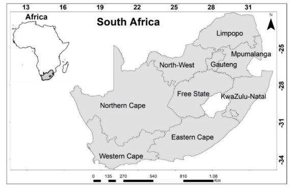
The global concentration of fine particulate matter (PM2.5) is experiencing an upward trend. This study investigates the utilization of space-time cubes to visualize and interpret PM2.5 data in South Africa over multiple temporal intervals spanning from 1998 to 2022. The findings indicated that the mean PM2.5 concentrations in Gauteng Province were the highest, with a value of 53 μg/m3 in 2010, whereas the lowest mean PM2.5 concentrations were seen in the Western Cape Province, with a value of 6.59 μg/m3 in 1999. In 2010, there was a rise in the average concentration of PM2.5 across all provinces. The increase might be attributed to South Africa being the host nation for the 2010 FIFA World Cup. In most provinces, there has been a general trend of decreasing PM2.5 concentrations over the previous decade. Nevertheless, the issue of PM2.5 remains a large reason for apprehension. The study also forecasts South Africa's PM2.5 levels until 2029 using simple curve fitting, exponential smoothing and forest-based models. Spatial analysis revealed that different areas require distinct models for accurate forecasts. The complexity of PM2.5 trends underscores the necessity for varied models and evaluation tools.
Citation: Tabaro H. Kabanda. Investigating PM2.5 pollution patterns in South Africa using space-time analysis[J]. AIMS Environmental Science, 2024, 11(3): 426-443. doi: 10.3934/environsci.2024021
The global concentration of fine particulate matter (PM2.5) is experiencing an upward trend. This study investigates the utilization of space-time cubes to visualize and interpret PM2.5 data in South Africa over multiple temporal intervals spanning from 1998 to 2022. The findings indicated that the mean PM2.5 concentrations in Gauteng Province were the highest, with a value of 53 μg/m3 in 2010, whereas the lowest mean PM2.5 concentrations were seen in the Western Cape Province, with a value of 6.59 μg/m3 in 1999. In 2010, there was a rise in the average concentration of PM2.5 across all provinces. The increase might be attributed to South Africa being the host nation for the 2010 FIFA World Cup. In most provinces, there has been a general trend of decreasing PM2.5 concentrations over the previous decade. Nevertheless, the issue of PM2.5 remains a large reason for apprehension. The study also forecasts South Africa's PM2.5 levels until 2029 using simple curve fitting, exponential smoothing and forest-based models. Spatial analysis revealed that different areas require distinct models for accurate forecasts. The complexity of PM2.5 trends underscores the necessity for varied models and evaluation tools.

| [1] |
Katoto PDMC, Byamungu L, Brand AS, et al. (2019) Ambient air pollution and health in Sub-Saharan Africa: Current evidence, perspectives and a call to action. Environ Res 173: 174–188. https://doi.org/10.1016/j.envres.2019.03.029 doi: 10.1016/j.envres.2019.03.029

|
| [2] |
Edlund KK, Killman F, Molnár P, et al. (2021) Health risk assessment of PM2.5 and PM2.5-bound trace elements in Thohoyandou, South Africa. Int J Environ Res 18: 1359. https://doi.org/10.3390/ijerph18031359 doi: 10.3390/ijerph18031359
|
| [3] | Indoor Quality Air. Air quality in South Africa, 2022. Available from: https://www.iqair.com/south-africa. |
| [4] | Zulu T, Aphane O, Audat T, et al. (2019) South Africa energy sector report. Available from: http://www.energy.gov.za/files/media/explained/2019-South-African-Energy-Sector-Report.pdf. |
| [5] |
Zhang R, Di B, Luo Y, et al. (2018) A nonparametric approach to filling gaps in satellite-retrieved aerosol optical depth for estimating ambient PM2.5 levels. Environ Pollut 243: 998–1007. https://doi.org/10.1016/j.envpol.2018.09.052 doi: 10.1016/j.envpol.2018.09.052
|
| [6] |
Yan JW, Tao F, Zhang SQ, et al. (2021) Spatiotemporal distribution characteristics and driving forces of PM2.5 in three urban agglomerations of the Yangtze River Economic Belt. Int J Env Res Pub He 18: 2222. https://doi.org/10.3390/ijerph18052222 doi: 10.3390/ijerph18052222
|
| [7] |
Chudnovsky AA, Koutrakis P, Kloog I, et al. (2014) Fine particulate matter predictions using high-resolution aerosol optical depth (AOD) retrievals. Atmos Environ 89: 189–198. https://doi.org/10.1016/j.atmosenv.2014.02.019 doi: 10.1016/j.atmosenv.2014.02.019
|
| [8] |
Stowell JD, Bi J, Al-Hamdan MZ, et al. (2020) Estimating PM2.5 in Southern California using satellite data: Factors that affect model performance. Environ Res Lett 15: 094004. https://doi.org/10.1088/1748-9326/ab9334 doi: 10.1088/1748-9326/ab9334
|
| [9] |
Hu X, Waller LA, Al-Hamdan MZ, et al. (2013) Estimating ground-level PM2.5 concentrations in the southeastern U.S. using geographically weighted regression. Environ Res 121: 1–10. https://doi.org/10.1016/j.envres.2012.11.003 doi: 10.1016/j.envres.2012.11.003
|
| [10] |
Kneen MA, Lary DJ, Harrison WA, et al. (2016) Interpretation of satellite retrievals of PM2.5 over the southern African Interior. Atmos Environ 128: 53–64. https://doi.org/10.1016/j.atmosenv.2015.12.016 doi: 10.1016/j.atmosenv.2015.12.016
|
| [11] |
Muyemeki L, Burger R, Piketh SJ (2020) Evaluating the potential of remote sensing imagery in mapping ground-level fine particulate matter (PM25) for the Vaal triangle priority area. Clean Air J 30: 1–7. https://doi.org/10.17159/caj/2020/30/1.8066 doi: 10.17159/caj/2020/30/1.8066
|
| [12] |
Hu X, Belle JH, Meng X, et al (2017) Estimating PM2.5 concentrations in the conterminous United States using the random forest approach. Environ Sci Technol 51: 6936–6944. https://doi.org/10.1021/acs.est.7b01210.s001 doi: 10.1021/acs.est.7b01210.s001
|
| [13] |
van Donkelaar A, Hammer M, Bindle L, et al. (2021) Monthly global estimates of fine particulate matter and their uncertainty. Environ Sci Technol 55: 15287–15300. https://doi.org/10.1021/acs.est.1c05309 doi: 10.1021/acs.est.1c05309
|
| [14] |
Knibbs LD, van Donkelaar A, Martin RV, et al. (2018) Satellite-based land-use regression for continental-scale long-term ambient PM2.5 exposure assessment in Australia. Environ Sci Technol 52: 12445–12455. https://doi.org/10.1021/acs.est.8b02328 doi: 10.1021/acs.est.8b02328
|
| [15] |
de Hoogh K, Gulliver J, van Donkelaar A, et al. (2016) Development of West-European PM2.5 and NO2 land use regression models incorporating satellite-derived and chemical transport modelling data. Environ Res 151: 1–10. https://doi.org/10.1016/j.envres.2016.07.005 doi: 10.1016/j.envres.2016.07.005
|
| [16] |
Hammer MS, van Donkelaar A, Li C, et al. (2020) Global estimates and long-term trends of fine particulate matter concentrations (1998–2018). Environ Sci Technol 54: 7879–7890. https://doi.org/10.1021/acs.est.0c01764 doi: 10.1021/acs.est.0c01764
|
| [17] |
van Donkelaar A, Martin RV, Li C, et al. (2019) Regional estimates of chemical composition of fine particulate matter using a combined geoscience-statistical method with information from satellites, models, and monitors. Environ Sci Technol 53: 2595. https://doi.org/10.1021/acs.est.8b06392 doi: 10.1021/acs.est.8b06392
|
| [18] |
Fenderson LE, Kovach AI, Llamas B (2020) Spatiotemporal landscape genetics: Investigating ecology and evolution through space and time. Mol Ecol 29: 218–246. https://doi.org/10.1111/mec.15315 doi: 10.1111/mec.15315
|
| [19] | Osman A, Owusu AB, Adu-Boahen K, et al. (2023) Space-time cube approach in analysing conflicts in Africa. Soc Sci Humanit Open 8. https://doi.org/10.1016/j.ssaho.2023.100557 |
| [20] |
Yoon J, Lee S (2021) Spatio-temporal patterns in pedestrian crashes and their determining factors: Application of a space-time cube analysis model. Accident Anal Prev 161. https://doi.org/10.1016/j.aap.2021.106291 doi: 10.1016/j.aap.2021.106291
|
| [21] |
Allen MJ, Allen TR, Davis C (2021) Exploring spatial patterns of Virginia tornadoes using kernel density and space-time cube analysis (1960–2019). ISPRS Int J Geo-Inf 10: 310. https://doi.org/10.3390/ijgi10050310 doi: 10.3390/ijgi10050310
|
| [22] |
Mo C, Tan D, Mai T, et al. (2020) An analysis of spatiotemporal pattern for COVID-19 in China based on space‐time cube. J Med Virol 92: 1587–1595. https://doi.org/10.1002/jmv.25834 doi: 10.1002/jmv.25834
|
| [23] | South African Yearbook (2021) South Africa Yearbook 2021/22. Available: https://www.gcis.gov.za/south-africa-yearbook-202122. |
| [24] | WUSTL (Washington University in St. Louis) (2022) Atmospheric composition analysis group-surface PM2.5. Available from: https://sites.wustl.edu/acag/datasets/surface-pm2-5/. |
| [25] | ESRI (2022) How Emerging Hot Spot Analysis Works. Available from: https://pro.arcgis.com/en/pro-app/latest/tool-reference/space-time-pattern-mining/learnmoreemerging.htm. |
| [26] |
Malik A, Kumar A, Pham QB, et al. (2020) Identification of EDI trend using Mann-Kendall and innovative trend methods (Uttarakhand, India). Arab J Geosci 13: 951. https://doi.org/10.1007/s12517-020-05926-2 doi: 10.1007/s12517-020-05926-2
|
| [27] |
Cui J, Liu Y, Sun J, et al. (2021) G-STC-M spatiotemporal analysis method for archaeological sites. ISPRS Int J Geo-Inf 10: 312. https://doi.org/10.3390/ijgi10050312 doi: 10.3390/ijgi10050312
|
| [28] |
Zhang H, Tripathi NK (2018) Geospatial hot spot analysis of lung cancer patients correlated to fine particulate matter (PM2.5) and industrial wind in Eastern Thailand. J Clean Prod 170: 407–424. https://doi.org/10.1016/j.jclepro.2017.09.185 doi: 10.1016/j.jclepro.2017.09.185
|
| [29] |
Harris NL, Goldman C, Gabris J, et al. (2017) Using spatial statistics to identify emerging hot spots of forest loss using spatial statistics to identify emerging hot spots of forest loss. Environ Res Lett 12. https://doi.org/10.1088/1748-9326/aa5a2f doi: 10.1088/1748-9326/aa5a2f
|
| [30] |
Wan Y, Beydoun MA (2007) The obesity epidemic in the United States—gender, Age, socioeconomic, racial/ethnic, and geographic characteristics: A systematic review and meta-regression analysis. Epidemiol Rev 29. https://doi.org/10.1093/epirev/mxm007 doi: 10.1093/epirev/mxm007
|
| [31] | Barazzetti L, Previtali M, Roncoroni F (2022) Visualisation and processing of structural monitoring data using space-time cubes, International Conference on Computational Science and Its Applications, Springer, Cham. https://doi.org/10.1007/978-3-031-10450-3_2 |
| [32] |
Zhou R, Chen H, Chen H, et al. (2021) Research on traffic situation analysis for urban road network through spatiotemporal data mining: A case study of Xi'an, China. IEEE Access 9: 75553–75567. https://doi.org/10.1109/access.2021.3082188 doi: 10.1109/access.2021.3082188
|
| [33] |
Cherchi E, Cirillo C (2010) Validation and forecasts in models estimated from multiday travel survey. Transport Res Rec 2175: 57–64. https://doi.org/10.3141/2175-07 doi: 10.3141/2175-07
|
| [34] | Arsham H (2020) Time-critical decision-making for business administration. Time Series Ana Bus Forecast. |
| [35] | ESRI (2023) Train time series forecasting model. Available from: https://pro.arcgis.com/en/pro-app/latest/tool-reference/geoai/train-time-series-forecasting-model.htm. |
| [36] |
Lapere R, Menut L, Mailler S, et al. (2020) Soccer games and record-breaking PM2.5 pollution events in Santiago, Chile. Atmos Chem Phys 20: 4681–4694. https://doi.org/10.5194/acp-20-4681-2020 doi: 10.5194/acp-20-4681-2020
|
| [37] | van der Merwe C (2010) The World Cup's 2, 7 MT carbon footprint and what's being done about it. Available from: https://www.engineeringnews.co.za/article/the-world-cups-27-million-ton-carbon-footprint-2010-01-22. |
| [38] | Paul M (2022) Different air under one sky: Almost everyone in South Africa breathes polluted air. Available from: https://www.downtoearth.org.in/news/health-in-africa/different-air-under-one-sky-almost-everyone-in-south-africa-breathes-polluted-air-84743. |
| [39] | Gray HA (2019) Air quality impacts and health effects due to sizeable stationary source emissions in and around South Africa's Mpumalanga highveld priority area, San Rafael, CA USA: Gray Sky Solutions. |
| [40] |
Zhang D, Du L, Wang W, et al. (2021) A machine learning model to estimate ambient PM2.5 concentrations in industrialized highveld region of South Africa. Remote Sens Environ 266: 112713. https://doi.org/10.1016/j.rse.2021.112713 doi: 10.1016/j.rse.2021.112713
|
| [41] |
Adeyemi A, Molnar P, Boman J, et al. (2022) Particulate matter (PM2.5) characterization, air quality level and origin of air masses in an urban background in Pretoria. Arch Environ Con Tox 83: 77–94. https://doi.org/10.1007/s00244-022-00937-4 doi: 10.1007/s00244-022-00937-4
|
| [42] |
Mollo VM, Nomngongo PN, Ramontja J (2022) Evaluation of surface water quality using various indices for heavy metals in Sasolburg, South Africa. Water 14: 2375. https://doi.org/10.3390/w1415237 doi: 10.3390/w1415237
|
| [43] |
Moreoane L, Mukwevho P, Burger R (2021) The quality of the first and second Vaal triangle airshed priority area air quality management plans. Clean Air J 31: 1–14. https://doi.org/10.17159/caj/2020/31/2.12178 doi: 10.17159/caj/2020/31/2.12178
|
| [44] |
Scorgie Y, Kneen A, Annegarn HJ, et al. (2003) Air pollution in the Vaal triangle-quantifying source contributions and identifying cost-effective solutions. Clean Air J 13: 5–18. https://doi.org/10.17159/caj/2003/13/2.7152 doi: 10.17159/caj/2003/13/2.7152
|
| [45] |
Venter AD, Beukes JP, Van Zyl PG (2012) An air quality assessment in the industrialised western Bushveld Igneous Complex, South Africa. S Afr J Sci 108: 1–10. https://doi.org/10.4102/sajs.v108i9/10.1059 doi: 10.4102/sajs.v108i9/10.1059
|
| [46] |
Matandirotya NR, Burger R (2023) An assessment of NO2 atmospheric air pollution over three cities in South Africa during 2020 COVID-19 pandemic. Air Qual Atmos Hlth 16: 263–276. https://doi.org/10.1007/s11869-022-01271-3 doi: 10.1007/s11869-022-01271-3
|
| [47] |
Shikwambana L, Mhangara P, Mbatha N (2020) Trend analysis and first time observations of sulphur dioxide and nitrogen dioxide in South Africa using TROPOMI/Sentinel-5 P data. Int J Appl Earth Obs 91. https://doi.org/10.1016/j.jag.2020.102130 doi: 10.1016/j.jag.2020.102130
|
| [48] | Department of Environmental Affairs (DEA) (2019) The second generation Vaal triangle airshed priority area air quality management plan: Draft baseline assessment report, Pretoria: DEA. |
| [49] | Norman R, Cairncross E, Witi J, et al. (2007) Estimating the burden of disease attributable to urban outdoor air pollution in South Africa in 2000. S Afr Med J 97: 748–753. |
| [50] |
Muyemeki L, Burger R, Piketh SJ, et al. (2021) Source apportionment of ambient PM10-25 and PM2.5 for the Vaal triangle, South Africa. S Afr J Sci 117: 1–11. https://doi.org/10.17159/sajs.2021/8617 doi: 10.17159/sajs.2021/8617
|
| [51] |
Oosthuizen MA, Mundackal AJ, Wright CY (2014) The prevalence of asthma among children in South Africa is increasing-is the need for medication increasing as well? A case study in the Vaal triangle. Clean Air J 24: 28–30. https://doi.org/10.17159/caj/2014/24/1.7050 doi: 10.17159/caj/2014/24/1.7050
|
| [52] |
Liu H, Yan G, Duan Z, et al. (2021) Intelligent modeling strategies for forecasting air quality time series: A review. Appl Soft Comput 102. https://doi.org/10.1016/j.asoc.2020.106957 doi: 10.1016/j.asoc.2020.106957
|
| [53] |
Gilliam RC, Hogrefe C, Rao ST (2006) New methods for evaluating meteorological models used in air quality applications. Atmos Environ 40: 5073–5086. https://doi.org/10.1016/j.atmosenv.2006.01.023 doi: 10.1016/j.atmosenv.2006.01.023
|


Figures(8) / Tables(3)

Tabaro H. Kabanda. Investigating PM2.5 pollution patterns in South Africa using space-time analysis[J]. AIMS Environmental Science, 2024, 11(3): 426-443. doi: 10.3934/environsci.2024021


 DownLoad: