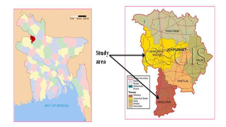
The discharge of untreated industrial effluents degraded water and soil, and the entire environment. The study aimed to evaluate the impacts of sugar mills effluent on the environment around the mills' area. A total of 120 effluents, soils, and water samples were collected three times a year over two years to analyze the physicochemical parameters. A field survey also was conducted on two hundred households of fourteen villages of the two Upazila in Joypurhat District of Bangladesh. The survey observed that majority of the people have negative opinions regarding the impacts of sugar mills effluents on fish, crops, and human health life. The higher BOD5 level in the effluents indicated that the decline in DO that the bacteria consumed the available oxygen in the water leading to the inability of fish and other aquatic organisms to survive in the water body. The study observed that the concentrations of Fe3+, Mn2+, and Pb2+ were found higher than the standard permissible limit of DoE-BD (2003) indicating the severe environmental degradation occurred in the areas. The study observed that the surface water, groundwater, and soil were contaminated through the discharge of sugar mills untreated effluents severely degraded the environment of the areas.
Citation: M.A. Rahim, M.G. Mostafa. Impact of sugar mills effluent on environment around mills area[J]. AIMS Environmental Science, 2021, 8(1): 86-99. doi: 10.3934/environsci.2021006
The discharge of untreated industrial effluents degraded water and soil, and the entire environment. The study aimed to evaluate the impacts of sugar mills effluent on the environment around the mills' area. A total of 120 effluents, soils, and water samples were collected three times a year over two years to analyze the physicochemical parameters. A field survey also was conducted on two hundred households of fourteen villages of the two Upazila in Joypurhat District of Bangladesh. The survey observed that majority of the people have negative opinions regarding the impacts of sugar mills effluents on fish, crops, and human health life. The higher BOD5 level in the effluents indicated that the decline in DO that the bacteria consumed the available oxygen in the water leading to the inability of fish and other aquatic organisms to survive in the water body. The study observed that the concentrations of Fe3+, Mn2+, and Pb2+ were found higher than the standard permissible limit of DoE-BD (2003) indicating the severe environmental degradation occurred in the areas. The study observed that the surface water, groundwater, and soil were contaminated through the discharge of sugar mills untreated effluents severely degraded the environment of the areas.

| [1] |
Islam MR, Mostafa MG (2020) Characterization of textile dyeing effluent and its treatment using polyaluminium chloride. J App Wat Sci 10:119. doi: 10.1007/s13201-020-01204-4

|
| [2] | Sattar MA, Rahaman AKM (2005) Heavy Metal Contaminations in the Environment, Sabdagussa Press, New York, 54pp. |
| [3] | Mostafa M.G, Helal Uddin, SM and ABMH Haque (2017) Assessment of Hydro-geochemistry and Groundwater Quality of Rajshahi City in Bangladesh. J App Wat Sci 7: 4663-4671. |
| [4] | Islam MR, Mostafa MG (2018) Textile Dyeing Effluents and Environment Concerns - A Review. J Env Sci & Nat Res 11: 131-144. |
| [5] |
Chowdhury M, Mostafa MG, Biswas TK, et al. (2015) Characterization of the Effluents from Leather Processing Industries. Env Procs 2: 173-187. doi: 10.1007/s40710-015-0065-7
|
| [6] |
Islam MS, Tanaka M (2004) Impact of pollution on coastal and marine ecosystems including coastal and marine fisheries and approach for management: a review and synthesis. Mar Pollut Bull 48: 624-649. doi: 10.1016/j.marpolbul.2003.12.004
|
| [7] |
Chowdhury M, Mostafa M G, Biswas TK, et al. (2013) Treatment of leather industrial effluents by filtration and coagulation processes. J Wat Res Ind 3: 11-22. doi: 10.1016/j.wri.2013.05.002
|
| [8] |
Dan'Azumi S, Bichi MH (2010) Industrial pollution and heavy metals profile of Challawa River in Kano, Nigeria. J App Sci Env Sani 5: 56-62. doi: 10.3923/jeasci.2010.56.63
|
| [9] |
Helal Uddin SM, Mostafa MG, Haque A (2011). Evaluation of groundwater quality and its suitability for drinking purpose in Rajshahi City, Bangladesh. Wat Sci and Tech: Wat Supply 11: 545-559. doi: 10.2166/ws.2011.079
|
| [10] | Qureshi AL, Mahessar AA, Leghari MEUH, et al. (2015) Impact of releasing wastewater of sugar industries into drainage system of LBOD, Sindh, Pakistan. Int J Env Sci and Dev 6: 381. |
| [11] | Sanjay KS (2005) Environmental pollution and sugar industry in India its management in: An appraisal. Sugar Tech 7: 77-81. |
| [12] | Banglapedia (2014) Sugar Industry (National Encyclopedia of Bangladesh) (Last visit: 20-1-2021). Website: http://en.banglapedia.org/index.php?title=Sugar_Industry#:~:text=Bangladesh%20now%20produces%20about%20150%2C000, tons%20of%20bagasse%20per%20year.&text=With%201.5%25%20of%20world%20production, the%20130%20sugar%20producing%20countries. |
| [13] | ETPI (Environmental Technology Program for Industry) (2001) Environmental report on sugar sector. Monthly Environ News 5: 11−27. |
| [14] | Hossain and Kabir (2010) Exploring the Nutrition and Health Benefits of Functional Foods. Web. https://doi.org/10.1007/s13201-020-01204-4. |
| [15] | APHA (American Public Health Association) (2012) Standard Methods for examination of water and wastewater. 22nd ed. Washington: Am. Pub. Health Assoc.; 2012, 1360 pp. ISBN 978-087553-013-0 http://www.standardmethods.org/ |
| [16] | IS (2000) Indian Standard methods of chemical analysis, Bureau of Indian Standards Manak Bhavan, 9 Bahadur Shah Zafar Marg New Delhi 110002. |
| [17] | NEQS (2000) National Environmental Quality Standards for municipal and liquid industrial effluents. |
| [18] | DoE-BD (Department of Environment, Bangladesh), (2003) A Compilation of Environmental Laws of Bangladesh. 212-214. |
| [19] | WHO (2011). Guidelines for Drinking-water Quality, 4rd (ISBN 978 92 4 154815 1). |
| [20] | Bhattacharjee S, Datta S, Bhattacharjee C (2007) Improvement of wastewater quality parameters by sedimentation followed by tertiary treatments, 212: 92-102 |
| [21] | Trivedi RK, Goel PK (1986) Chemical and biological methods for water pollution studies. Environ Pub Karad. |
| [22] | Saifi S, Mehmood T (2011) Effects of socioeconomic status on students' achievement. Int J Social Sci Edu 1: 119-128. |
| [23] |
Akan JC, Moses EA, Ogugbuaja VO (2007) Determination of pollution levels in Mario Jose Tannery Effluents from Kano Metropolice, Nigeria. J Appl Sci 7: 527-530. doi: 10.3923/jas.2007.527.530
|
| [24] |
Buekers J, Van Laer L, Amery F, et al. (2007) Role of soil constituents in fixation of soluble Zn, Cu, Ni and Cd added to soils. Euro J Soil Sci 58: 1514-1524. doi: 10.1111/j.1365-2389.2007.00958.x
|
| [25] |
Levy DB, Barbarick KA, Siemer EG, et al. (1992) Distribution and partitioning of trace metals in contaminated soils near Leadville, Colorado. J Environ Qual 21: 185-195. doi: 10.2134/jeq1992.00472425002100020006x
|
| [26] | BBS (2011) Bangladesh National Drinking water quality survey of 2009. Bangladesh Bureau of Statistics, Planning Division, Ministry of Planning, Government of the People's Republic of Bangladesh, 192pp. |
| [27] | Flora SJS, Flora G, Saxena G (2006) Environmental occurrence, health effects and management of lead poisoning. In: José, S. C, José, S., eds. Lead. Amsterdam: Elsevier Science B.V., pp. 158-228. |
| [28] | Saha MK, Ahmed SJ, Sheikh MAH, et al. (2020) Occupational and environmental health hazards in brick kilns. J Air Poll Health 5: 135-146. |
| [29] | AAP (American Academy of Pediatrics) (2005) Lead Exposure in Children: Prevention, Detection, and Management: Web. http://pediatrics.aappublications.org/content/116/4/1036.full |

Figures(2) / Tables(7)

M.A. Rahim, M.G. Mostafa. Impact of sugar mills effluent on environment around mills area[J]. AIMS Environmental Science, 2021, 8(1): 86-99. doi: 10.3934/environsci.2021006


 DownLoad: