A comprehensive review of solar thermal desalination technologies for freshwater production

Laveet Kumar; Jahanzaib Soomro; Hafeez Khoharo; Mamdouh El Haj Assad; Laveet Kumar; Jahanzaib Soomro; Hafeez Khoharo; Mamdouh El Haj Assad

doi:10.3934/energy.2023016

AIMS Energy

2023, Volume 11, Issue 2: 293-318. doi: 10.3934/energy.2023016

Previous Article Next Article

Review Special Issues

A comprehensive review of solar thermal desalination technologies for freshwater production

1.
Department of Mechanical Engineering, Mehran University of Engineering and Technology, Jamshoro, Pakistan
2.
Department of Sustainable and Renewable Energy Engineering, University of Sharjah, Sharjah, United Arab Emirates

Received: 09 November 2022 Revised: 13 March 2023 Accepted: 14 March 2023 Published: 23 March 2023

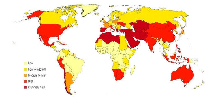
This review is inspired by the increasing shortage of fresh water in areas of the world, and is written in response to the expanding demand for sustainable technologies due to the prevailing crisis of depleting natural water resources. It focuses on comprehending different solar energy-based technologies. Since the increasing population has resulted in the rising demand for freshwater, desalination installation volume is rapidly increasing globally. Conventional ways of desalination technologies involve the use of fossil fuels to extract thermal energy which imparts adverse impacts on the environment. To lessen the carbon footprint left by energy-intensive desalination processes, the emphasis has shifted to using renewable energy sources to drive desalination systems. The growing interest in combining solar energy with desalination with an emphasis on increasing energy efficiency has been sparked by the rapid advancements in solar energy technology, particularly solar thermal. This review paper aims to reflect various developments in solar thermal desalination technologies and presents prospects of solar energy-based desalination techniques. This paper reviews direct and indirect desalination techniques coupled with solar energy, and goes on to explain recent trends in technologies. This review also summarizes the emerging trends in the field of solar thermal desalination technologies. The use of nanoparticles and photo-thermal materials for localized heating in solar desalination systems has decreased energy consumption and enhanced the efficiency of the system. Solar power combined with emerging processes like membrane distillation (MD) has also a recent resurgence.

Keywords:

Citation: Laveet Kumar, Jahanzaib Soomro, Hafeez Khoharo, Mamdouh El Haj Assad. A comprehensive review of solar thermal desalination technologies for freshwater production[J]. AIMS Energy, 2023, 11(2): 293-318. doi: 10.3934/energy.2023016

Related Papers:

[1]	Xiaoling Chen, Xingfa Zhang, Yuan Li, Qiang Xiong . Daily LGARCH model estimation using high frequency data. Data Science in Finance and Economics, 2021, 1(2): 165-179. doi: 10.3934/DSFE.2021009
[2]	Paarth Thadani . Financial forecasting using stochastic models: reference from multi-commodity exchange of India. Data Science in Finance and Economics, 2021, 1(3): 196-214. doi: 10.3934/DSFE.2021011
[3]	Kexian Zhang, Min Hong . Forecasting crude oil price using LSTM neural networks. Data Science in Finance and Economics, 2022, 2(3): 163-180. doi: 10.3934/DSFE.2022008
[4]	Moses Khumalo, Hopolang Mashele, Modisane Seitshiro . Quantification of the stock market value at risk by using FIAPARCH, HYGARCH and FIGARCH models. Data Science in Finance and Economics, 2023, 3(4): 380-400. doi: 10.3934/DSFE.2023022
[5]	Samuel Asante Gyamerah, Collins Abaitey . Modelling and forecasting the volatility of bitcoin futures: the role of distributional assumption in GARCH models. Data Science in Finance and Economics, 2022, 2(3): 321-334. doi: 10.3934/DSFE.2022016
[6]	Alejandro Rodriguez Dominguez, Om Hari Yadav . A causal interactions indicator between two time series using extreme variations in the first eigenvalue of lagged correlation matrices. Data Science in Finance and Economics, 2024, 4(3): 422-445. doi: 10.3934/DSFE.2024018
[7]	Wojciech Kurylek . Are Natural Language Processing methods applicable to EPS forecasting in Poland?. Data Science in Finance and Economics, 2025, 5(1): 35-52. doi: 10.3934/DSFE.2025003
[8]	Nitesha Dwarika . The risk-return relationship in South Africa: tail optimization of the GARCH-M approach. Data Science in Finance and Economics, 2022, 2(4): 391-415. doi: 10.3934/DSFE.2022020
[9]	Mohamed F. Abd El-Aal . Analysis Factors Affecting Egyptian Inflation Based on Machine Learning Algorithms. Data Science in Finance and Economics, 2023, 3(3): 285-304. doi: 10.3934/DSFE.2023017
[10]	Xiaozheng Lin, Meiqing Wang, Choi-Hong Lai . A modification term for Black-Scholes model based on discrepancy calibrated with real market data. Data Science in Finance and Economics, 2021, 1(4): 313-326. doi: 10.3934/DSFE.2021017

Abstract

1. Introduction

Estimating foreign exchange rate (FX) volatility is a core risk management activity for financial institutions, corporates and regulators. The subject has been extensively investigated among both practitioners and scientific researchers, and several alternative models exist. Among the most prominent are the models belonging to GARCH and stochastic volatility classes. However, the true value of volatility cannot be directly observed. Hence, volatility must be estimated, inevitably with error. This constitutes a fundamental problem in implementing parametric models, especially in the context of high-frequency data. Andersen and Bollerslev (1998) proposed using realized volatility, as derived from high-frequency data, to accurately measure the true latent integrated volatility. This approach has gained attention for volatility modeling in markets where tick-level data is available (Andersen et al., 2013). Andersen et al. (2003) suggest fractionally integrated ARFIMA models in this context. Still, the long-memory HAR (heterogeneous autoregressive) model of is arguably the most widely used to capture the high persistence typically observed in realized volatility of financial prices. The HAR model is relatively simple and easy to estimate. In empirical applications, the model tends to perform better than GARCH and stochastic volatility models possibly due to the sensitivity of tightly parameterized volatility models to minor model misspecifications (). Although realized volatility $(RV)$ is a consistent estimator of the true latent volatility, it is subject to measurement error in empirical finite samples. Hence, $RV$ will not only reflect the true latent integrated volatility $(IV)$ , but also additional measurement errors. Bollerslev et al. (2016) propose utilizing higher-order realized moments of the realized distribution to approximate these measurement errors. More specifically, Bollerslev et al. (2016) propose the HARQ-model, which augments the HAR model with realized quarticity as an additional covariate.

The empirical performance of the HARQ and related extensions has been extensively studied. The focus has predominantly been on equity markets. A majority of the studies analyze U.S. data; see Bollerslev et al. (2016); Clements, A. and Preve, D. (2021); Pascalau and Poirier (2023); Andersen et al. (2023) and others. Liu et al. (2018) and Wang et al. (2020) investigate Chinese equity markets, whereas Liang et al. (2022); Ma et al. (2019) analyse international data. Bitcoin and electricity markets have attracted some attention; see, for instance, Shen et al. (2020); Qieu et al. (2021), and Qu et al. (2018).

Empirical applications of the HARQ model in the context of foreign exchange rate risk are sparse. Lyócsa et al. (2016) find that the standard HAR model rarely is outperformed by less parsimonious specifications on CZKEUR, PLZEUR, and HUFEUR data. Plíhal et al. (2021) and Rokicka and Kudła (2020) estimate the HARQ model on EURUSD and EURGBP data, respectively. Their focus is different from ours, as they investigate the incremental predictive power of implied volatility for a broad class of HAR models. In a similar vein, Götz (2023) and Lyócsa et al. (2024) utilize the HARQ model for the purpose of estimating foreign exchange rate tail risk.

Using updated tick-level data from two major currency pairs, EURUSD and USDJPY, this paper documents the relevance of realized quarticity for improving volatility estimates across varying forecasting horizons. These results are robust across estimation windows, evaluation metrics, and model specifications.

2. Materials and method

2.1. Data

We use high-frequency intraday ticklevel spot data, publicly available at DukasCopy^* The sample period is 1. January 2010 to 31. December 2022. Liu et al. (2015) investigate the optimal intraday sampling frequency across a significant number of asset classes and find that 5-min intervals usually outperform others. Hence, as common in the literature, we estimate the realized volatility from 5-minute returns.

^*This data source is also used by Plíhal et al. (2021), Risstad et al. (2023) and Lyócsa et al. (2024), among others.

To filter tick-level data, we follow a two-step cleaning procedure based on the recommendations by Barndorff-Nielsen et al. (2009). Initially, we eliminate data entries that exhibit any of the following issues: (i) absence of quotes, (ii) a negative bid-ask spread, (iii) a bid-ask spread exceeding 50 times the median spread of the day, or (iv) a mid-quote deviation beyond ten mean absolute deviations from a centered mean (computed excluding the current observation from a window of 25 observations before and after). Following this, we calculate the mid-quotes as the average of the bid and ask quotes and then resample the data at 5-minute intervals.

We compute the consistent estimator of the true latent time- $t$ variance from

$\begin{equation} RV^{2}_{t} \equiv \sum\limits^{M}_{t = 1} r^{2}_{t, i}, \end{equation}$

(1)

where $M = 1/\Delta$ , and the $\Delta$ -period intraday return is $r_{t, i} \equiv \log(S_{t-1+i\times\Delta}) - \log(S_{t-1+(i-1)\times\Delta})$ , where $S$ is the spot exchange rate. Analogously, the multi $(h)$ -period realized variance estimator is

$\begin{equation} RV^{2}_{t-1, t-h} = \frac{1}{h} \sum\limits_{i = 1}^{h}RV^{2}_{t-h}. \end{equation}$

(2)

Setting $h = 5$ and $h = 22$ yields weekly and monthly estimates, respectively.

Table 1 displays descriptive statistics for daily realized variances, as computed from (1).

Table 1. Realized Variance (daily).

	Min	Mean	Median	Max	$\rho_1$
EURUSD	0.1746	3.0606	2.2832	59.4513	0.5529
USDJPY	0.1018	3.2460	2.0096	168.0264	0.2860
The table contains summary statistics for the daily $R V \mathrm{~s}$ for EURUSD and USDJPY. $\rho_1$ is the standard first order autocorrelation coefficient. Sample period: 1. January 2010 to 31. December 2022.

| Show Table

DownLoad: CSV

2.2. The HARQ models

To represent the long-memory dynamic dependencies in volatility, Corsi (2009) proposed using daily, weekly, and monthly lags of realized volatility as covariates. The original HAR model is defined as

$\begin{equation} R V_{t} = \beta_{0}+\beta_{1} R V_{t-1}+\beta_{2} R V_{t-1 \mid t-5}+\beta_{3} R V_{t-1 \mid t-22}+u_{t}, \end{equation}$

(3)

where $RV$ is computed from (1) and (2). If the variables in (2.2) contain measurement errors, the beta coefficients will be affected. Bollerslev et al. (2016) suggests two measures to alleviate this. First, they include a proxy for measurement error as an additional explanatory variable. Furthermore, they directly adjust the coefficients in proportion to the magnitude of the measurement errors:

$\begin{aligned} R V_{t} = & \beta_{0}+\underbrace{\left(\beta_{1}+\beta_{1 Q} R Q_{t-1}^{1 / 2}\right)}_{\beta_{1, t}} R V_{t-1} \\ & +\underbrace{\left(\beta_{2}+\beta_{2 Q} R Q_{t-1 \mid t-5}^{1 / 2}\right)}_{\beta_{2, t}} R V_{t-1 \mid t-5} \\ & +\underbrace{\left(\beta_{3}+\beta_{3 Q} R Q_{t-1 \mid t-22}^{1 / 2}\right)}_{\beta_{3, t}} R V_{t-1 \mid t-22}+u_{t}, \end{aligned}$

where realized quarticity $RQ$ is defined as

$\begin{equation} R Q_{t} \equiv \frac{M}{3} \sum\limits_{i = 1}^{M} r_{t, i}^{4} \end{equation}$

(4)

The full HARQ model in (2.2) adjusts the coefficients on all lags of $RV$ . A reasonable conjecture is that measurement errors in realized volatilities tend to diminish at longer forecast horizons, as these errors are diversified over time. This suggests that measurement errors in daily lagged realized volatilities are likely to be relatively more important. Motivated by this Bollerslev et al. (2016) specify the HARQ model as

$\begin{equation} \begin{aligned} R V_{t} = & \beta_{0}+\underbrace{\left(\beta_{1}+\beta_{1 Q} R Q_{t-1}^{1 / 2}\right)}_{\beta_{1, t}} R V_{t-1}+\beta_{2} R V_{t-1 \mid t-5} \\ & +\beta_{3} R V_{t-1 \mid t-22}+u_{t} . \end{aligned} \end{equation}$

(5)

Although there is no reason to expect that autoregressive models of order one will be able to accurately capture long memory in realized volatility, we estimate AR(1) models as a point of reference. The AR and ARQ models are defined as

$\begin{equation} \begin{aligned} R V_{t} = \beta_{0}+\beta_{1} RV_{t-1}+u_{t}. \end{aligned} \end{equation}$

(6)

and

$\begin{equation} \begin{aligned} R V_{t} = \beta_{0}+\underbrace{\left(\beta_{1}+\beta_{1 Q} R Q_{t-1}^{1 / 2}\right)}_{\beta_{1, t}} R V_{t-1}+u_{t}. \end{aligned} \end{equation}$

(7)

in equations (6) and (7), respectively.

3. Results and discussion

Due to noisy data and related estimation errors, forecasts from realized volatility models might occasionally appear as unreasonably high or low. Thus, in line with Swanson et al. (1997) and Bollerslev et al. (2016), we filter forecasts from all models so that any forecast outside the empirical distribution of the estimation sample is replaced by the sample mean.

3.1. In-sample estimation results

reports in-sample parameter estimates for the ARQ, HARQ, and HARQ-F models, along with the benchmark AR and ARQ models, for one-day ahead EURUSD (upper panel) and USDJPY (lower panel) volatility forecasts. Robust standard errors (s.e.) are computed as proposed by . $R^{2}$ , $MSE$ , and $QLIKE$ are displayed at the bottom of each panel.

Table 2. In-sample estimation results, one-day-ahead volatility forecasts.

EURUSD	AR	HAR	ARQ	HARQ	HARQ-F
$\beta_{0}$	$1.3663^*$	$0.3961^*$	$0.7428^*$	$0.2785^*$	$-$ 0.0651
s.e.	0.1843	0.0598	0.0969	0.0586	0.0685
$\beta_{1}$	$0.5530^{*}$	$0.2364^{*}$	$0.7903^{*}$	$0.4349^{*}$	$0.3740^{*}$
s.e.	0.0653	0.0730	0.0388	0.0754	0.0792
$\beta_{2}$		$0.3767^{*}$		$0.3072^{*}$	$0.4613^{*}$
s.e.		0.0717		0.0697	0.1031
$\beta_{3}$		$0.2572^{*}$		$0.1850^{*}$	$0.2398^{*}$
s.e.		0.0532		0.0515	0.0822
$\beta_{1 Q}$			$-2.4914^{*}$	$-1.3708^{*}$	$-0.9710^{*}$
s.e.			0.3377	0.1939	0.2266
$\beta_{2 Q}$					$-1.7578^{***}$
s.e.					0.8706
$\beta_{3 Q}$					$-3.9819^{*}$
s.e.					1.1618
$R^{2}$	0.3058	0.3956	0.3685	0.4101	0.4166
$MSE$	6.3005	5.4852	5.7315	5.3538	5.2950
$QLIKE$	0.1647	0.1230	0.1540	0.1217	0.1199
USDJPY	AR	HAR	ARQ	HARQ	HARQ-F
$\beta_{0}$	$2.3073^{*}$	$1.0682^{*}$	$1.3537^{*}$	$0.7811^{*}$	$0.5218^{*}$
s.e.	0.2362	0.1381	0.2207	0.1429	0.1328
$\beta_{1}$	$0.2854^{*}$	$0.1819^{*'}$	$0.6180^{*}$	$0.5177^{***}$	$0.4416^{*}$
s.e.	0.0804	0.0806	0.0853	0.1106	0.1260
$\beta_{2}$		$0.1441^{**}$		0.0542	$0.2345^{***}$
s.e.		0.0585		0.0543	0.1072
$\beta_{3}$		$0.3443^{*}$		$0.2188^{*}$	$0.2228^{*}$
s.e.		0.0499		0.0493	0.0658
$\beta_{1 Q}$			$-0.2295^{*}$	$-0.1967^{*}$	$-0.1526^{*}$
s.e.			0.0318	0.0386	0.0476
$\beta_{2 Q}$					$-0.2296^{**}$
s.e.					0.0849
$\beta_{3 Q}$					$-0.3573^{*}$
s.e.					0.1142
$R^{2}$	0.0814	0.1154	0.1489	0.1581	0.1642
$MSE$	33.6096	32.3668	31.1409	30.8063	30.5818
$QLIKE$	0.3214	0.2561	0.2663	0.2377	0.2242
Note: The table contains in-sample parameter estimates and corresponding standard errors (), together with $R^{2}$ . $MSE$ and $QLIKE$ computed from (12) and (13). Superscripts , , and ** represent statistical significance in a two-sided t-test at 1%, 5% and 10% levels, respectively.

| Show Table

DownLoad: CSV

The coefficients $\beta_{1 Q}$ are negative and exhibit strong statistical significance, aligning with the hypothesis that $RQ$ represents time-varying measurement error. When comparing the autoregressive (AR) coefficient of the AR model to the autoregressive parameters in the ARQ model, the AR coefficient is markedly lower, reflecting the difference in in persistence between the models.

In the comparative analysis of the HAR and HARQ models applied to both currency pairs, the HAR model assigns more emphasis to the weekly and monthly lags, which are generally less sensitive to measurement errors. In contrast, the HARQ model typically assigns a higher weight to the daily lag. However, when measurement errors are substantial, the HARQ model reduces the weight on the daily lag to accommodate the time-varying nature of the measurement errors in the daily realized volatility ( $RV$ ). The flexible version of this model, the HARQ-F, allows for variability in the weekly and monthly lags, resulting in slightly altered parameters compared to the standard HARQ model. Notably, the coefficients $\beta_{2 Q}$ and $\beta_{3 Q}$ in the HARQ-F model are statistically significant, and this model demonstrates a modest enhancement in in-sample fit relative to the HARQ model.

3.2. Out-of-sample forecasting results

To further assess the out-of-sample performance of the HARQ model, we consider three alternative HAR type specifications. More specifically, we include both the HAR-with-Jumps (HAR-J) and the Continuous-HAR (CHAR) proposed by Andersen et al. (2007), as well as the SHAR model proposed by Patton and Sheppard (2015), in the forecasting comparisons. Based on the Bi-Power Variation (BPV) measure of Barndorff-Nielsen and Shephard (2004), HAR-J and CHAR decompose the total variation into a continuous and a discontinuous (jump) part.

The HAR-J model augments the standard HAR model with a measure of the jump variation;

$\begin{equation} \begin{aligned} R V_{t} = & \beta_{0}+\beta_{1} R V_{t-1}+\beta_{2} R V_{t-1 \mid t-5}+\beta_{3} R V_{t-1 \mid t-22} \\ & +\beta_{J} J_{t-1}+u_{t}, \end{aligned} \end{equation}$

(8)

where $J_{t} \equiv \max \left[R V_{t}-B P V_{t}, 0\right]$ , and the $B P V$ measure is defined as,

$\begin{equation} BPV_{t} \equiv \mu_{1}^{-2} \sum\limits_{i = 1}^{M-1}\left|r_{t, i}\right|\left|r_{t, i+1}\right|, \end{equation}$

(9)

with $\mu_{1} = \sqrt{2 / \pi} = \mathbb{E}(|Z|)$ , and $Z$ is a standard normal random variable.

The CHAR model includes measures of the continuous component of the total variation as covariates;

$\begin{equation} R V_{t} = \beta_{0}+\beta_{1} B P V_{t-1}+\beta_{2} B P V_{t-1 \mid t-5}+\beta_{3} B P V_{t-1 \mid t-22}+u_{t}. \end{equation}$

(10)

Inspired by the semivariation measures of , propose the SHAR model, which, in contrast to the HAR model, effectively allows for asymmetric responses in volatility forecasts from negative and positive intraday returns. More specifically, when $R V_{t}^{-} \equiv \sum_{i = 1}^{M} r_{t, i}^{2} \mathbb{I}_{\left\{r_{t, i} < 0\right\}}$ and $R V_{t}^{+} \equiv \; \sum_{i = 1}^{M} r_{t, i}^{2} \mathbb{I}_{\left\{r_{t, i} > 0\right\}}$ , the SHAR model is defined as:

$\begin{equation} \begin{aligned} R V_{t} = & \beta_{0}+\beta_{1}^{+} R V_{t-1}^{+}+\beta_{1}^{-} R V_{t-1}^{-}+\beta_{2} R V_{t-1 \mid t-5} \\ & +\beta_{3} R V_{t-1 \mid t-22}+u_{t} . \end{aligned} \end{equation}$

(11)

To evaluate model performance, we consider the mean squared error (MSE) and the QLIKE loss, which, according to Patton (2011), both are robust to noise. MSE is defined as

$\begin{equation} MSE(RV_{t}, F_{t}) \equiv (RV_{t}-F_{t})^2, \end{equation}$

(12)

where $F_{t}$ refers to the one-period direct forecast. QLIKE is defined as

$\begin{equation} QLIKE(RV_{t}, F_{t}) \equiv \frac{RV_{t}}{F_{t}} - \ln\left(\frac{RV_{t}}{F_{t}}\right) -1. \end{equation}$

(13)

3.2.1. Daily forecasting horizon

contains one-day-ahead forecasts for EURUSD and USDJPY. The table reports model performance, expressed as model loss normalized by the loss of the HAR model. Each row reflects a combination of estimation window and loss function. The lowest ratio on each row, highlighting the best, performing model, is in bold. We evaluate the models using both a rolling window $(RW)$ and an expanding window $(EW)$ . In both cases, forecasts are derived from model parameters re-estimated each day with a fixed length $RW$ comprised of the previous 1000 days, as well as an $EW$ using all of the available observations. The sample sizes for $EW$ thus range from 1000 to 3201 days. The results are consistent in that the HARQ-F model is the best performer for both currency pairs and across loss functions and estimation windows. The HARQ model is closest to HARQ-F. Neither HAR-J, CHAR, nor SHAR appear to consistently improve upon the standard HAR model.

Table 3. Out-of-sample forecast losses, one-day-ahead volatility forecasts.

EURUSD	AR	HAR	HAR-J	CHAR	SHAR	ARQ	HARQ	HARQ-F
MSE-RW	1.1483	1.0000	1.0088	0.9945	1.0080	1.0311	0.9759	0.9655^*
MSE-EW	1.1619	1.0000	0.9984	0.9908	1.0050	1.02660	0.9742	0.9720^*
QLIKE-RW	1.3153	1.0000	0.9907	0.9813	1.0078	1.1575	0.9767	0.9582^*
QLIKE-EW	1.3915	1.0000	0.9907	0.9944	1.0052	1.1927	0.9952	0.9721^**
USDJPY	AR	HAR	HAR-J	CHAR	SHAR	ARQ	HARQ	HARQ-F
MSE-RW	1.0502	1.0000	1.0053	0.9979	1.0238	0.8907	0.8885	0.8832^*
MSE-EW	1.0475	1.0000	1.0243	1.0133	1.0515	0.9558	0.9446	0.9376^*
QLIKE-RW	1.2320	1.0000	1.0748	0.9944	0.9811	0.9482	0.8824	0.8667^*
QLIKE-EW	1.3066	1.0000	1.0023	0.9800	0.9941	1.0039	0.8949	0.8519^*
Note: Model performance, expressed as model loss normalized by the loss of the HAR model. Each row reflects a combination of estimation window and loss function. Ratio for the best performing model on each row in bold. Corresponding asterix * and ** denote 1% and 5% confidence levels from Diebold-Mariano test for one-sided tests of superior performance of the best performing model compared to the HAR model.

| Show Table

DownLoad: CSV

Judging from , it is beneficial to include RQ as an explanatory variable when RV is measured inaccurately. However, precise measurement of RV becomes more difficult when RV is high, inducing a positive correlation between RV and RQ. At the same time, high $RV$ often coincides with jumps. To clarify whether the performance of RQ-based models is due to jump dynamics, further segments the results in into forecasts for days when the previous day's $RQ$ was very high (Top 5% RQ, Table 4b) and the remaining sample (Bottom 95% RQ, Table 4a). As this breakdown shows, the RQ-based models perform relatively well also during periods of non-extreme heteroscedasticity of RQ.

Table 4. Stratified one-day-ahead out-of-sample forecast losses.

(a) Bottom 95% RQ
EURUSD	AR	HAR	HAR-J	CHAR	SHAR	ARQ	HARQ	HARQ-F
MSE-RW	1.1156	1.0000	0.9937	0.9907	1.0021	1.0636	0.9925	0.9794
MSE-IW	1.1175	1.0000	0.9887	0.9885	1.0020	1.0711	0.9967	0.9866
QLIKE-RW	1.3299	1.0000	0.9975	0.9855	1.0071	1.1598	0.9745	0.9555
QLIKE-IW	1.4108	1.0000	0.9956	0.9980	1.0055	1.1995	0.9944	0.9720
heightUSDJPY	AR	HAR	HAR-J	CHAR	SHAR	ARQ	HARQ	HARQ-F
MSE-RW	1.0330	1.0000	1.0146	0.9984	0.9940	0.9592	0.9526	0.9495
MSE-IW	1.0590	1.0000	0.9962	0.9925	1.0001	0.9849	0.9681	0.9601
QLIKE-RW	1.2507	1.0000	1.1353	0.9877	0.9829	0.9542	0.8797	0.8450
QLIKE-IW	1.3266	1.0000	0.9883	0.9734	0.9993	1.0100	0.8887	0.8434
(b) Top 5% RQ
EURUSD	AR	HAR	HAR-J	CHAR	SHAR	ARQ	HARQ	HARQ-F
MSE-RW	1.2276	1.0000	1.0453	1.0036	1.0225	0.9523	0.9355	0.9316
MSE-IW	1.2642	1.0000	1.0206	0.9960	1.0121	0.9218	0.9224	0.9382
QLIKE-RW	1.0876	1.0000	0.8851	0.9152	1.0186	1.1223	1.0116	0.9996
QLIKE-IW	1.0902	1.0000	0.9141	0.9389	1.0006	1.0856	1.0081	0.9745
USDJPY	AR	HAR	HAR-J	CHAR	SHAR	ARQ	HARQ	HARQ-F
MSE-RW	1.0674	1.0000	1.0025	0.9974	1.0535	0.9425	0.8700	0.8518
MSE-IW	1.0347	1.0000	1.0566	1.0365	1.1090	0.9246	0.9183	0.9126
QLIKE-RW	1.0202	1.0000	1.5755	1.0697	0.9601	0.8803	0.9135	0.9999
QLIKE-IW	1.0544	1.0000	1.1789	1.0628	0.9279	0.9278	0.9730	0.9588
Note: The table segments the results in according to $RQ$ . The bottom panel shows the ratios for days following a value of $RQ$ in the top $5\%$ . The top panel shows the results for the remaining $95\%$ of sample. Ratio for the best performing model on each row in bold.

| Show Table

DownLoad: CSV

3.2.2. Longer forecast horizons

In practitioner applications, longer forecasts than one day are often of interest. We now extend our analysis to weekly and monthly horizons, using direct forecasts. The daily forecast analysis in subsubsection 3.2.1 indicates the lag order of RQ plays an important role in forecast accuracy. Hence, following Bollerslev et al. (2016), we consider the HARQ-h model, and adjust the lag corresponding to the specific forecast horizon only. Specifically, for the weekly and monthly forecasts analysed here, the relevant HARQ-h specifications become

$\begin{equation} \begin{aligned} R V_{t+4 \mid t} = & \beta_{0}+\beta_{1} R V_{t-1}+\underbrace{\left(\beta_{2}+\beta_{2 Q} R Q_{t-1 \mid t-5}^{1 / 2}\right)}_{\beta_{2, t}} R V_{t-1 \mid t-5} \\ & +\beta_{3} R V_{t-1 \mid t-22}+u_{t} \end{aligned} \end{equation}$

(14)

and

$\begin{equation} \begin{aligned} R V_{t+21 \mid t} = & \beta_{0}+\beta_{1} R V_{t-1}+\beta_{2} R V_{t-1 \mid t-5}+u_{t}, \\ & +\underbrace{\left(\beta_{3}+\beta_{3 Q} R Q_{t-1 \mid t-22}^{1 / 2}\right)}_{\beta_{3, t}} R V_{t-1 \mid t-22}+u_{t}, \end{aligned} \end{equation}$

(15)

respectively.

presents in-sample parameter estimates across model specifications. The patterns observed here closely resemble those of the daily estimates detailed in . All coefficients on RQ ( $\beta_{1Q}, \beta_{2Q}, \beta_{3Q}$ ) are negative, except for the $(h = 22)$ lag statistically significant. This indicates that capturing measurement errors is relevant also for forecast horizons beyond one day. The HARQ model consistently allocates greater weight to the daily lag compared to the standard HAR model. Similarly, the HARQ-h model predominantly allocates its weight towards the time-varying lag. The weights of the HARQ-F model on the different lags are relatively more stable when compared to the HARQ-h model.

Table 5. In-sample weekly and monthly model estimates.

(a) EURUSD
	Weekly						Monthly
	AR	ARQ	HAR	HARQ	HARQ-F	HARQ-h	AR	ARQ	HAR	HARQ	HARQ-F	HARQ-h
$\beta_{0}$	$0.8646^{*}$	$0.2634^{*}$	$0.5680^{*}$	$0.4758^{*}$	-0.0250	$0.2275^{**}$	$1.6388^{*}$	$0.9642^{*}$	$0.9269^{*}$	$0.8452^{*}$	0.2328	0.2153
s.e.	0.1345	0.0927	0.0997	0.0882	0.0895	0.0861	0.1806	0.1840	0.2246	0.2099	0.2080	0.2093
$\beta_{1}$	$0.7168^{*}$	$0.9620^{*}$	$0.1194^{*}$	$0.2752^{*}$	$0.1836^{*}$	$0.1181^{*}$	$0.4616^{*}$	$0.7373^{*}$	$0.0717^{*}$	$0.2097^{*}$	$0.1131^{*}$	$0.0646^{*}$
s.e.	0.0480	0.0400	0.0264	0.0395	0.0269	0.0214	0.0564	0.0616	0.0205	0.0401	0.0248	0.0185
$\beta_{2}$			$0.3938^{*}$	$0.3395^{*}$	$0.5777^{*}$	$0.7635^{*}$			$0.2091^{*}$	$0.1606^{*}$	$0.3706^{*}$	$0.2176^{*}$
s.e.			0.0887	0.0881	0.1282	0.1139			0.0587	0.0554	0.0962	0.0563
$\beta_{3}$			$0.3008^{*}$	$0.2440^{*}$	$0.3131^{**}$	0.0876			$0.4163^{*}$	$0.3661^{*}$	$0.5153^{*}$	$0.7179^{*}$
s.e.			0.0880	0.0817	0.1275	0.0940			0.1186	0.1174	0.1498	0.1106
$\beta_{1Q}$		$-5.4876^{*}$		$-1.0749^{*}$	$-0.4728^{*}$			$-6.1534^{*}$		$-0.9499^{*}$	$-0.3246^{*}$
s.e.		0.4817		0.1377	0.1005			0.9900		0.1815	0.0846
$\beta_{2Q}$					$-2.7357^{*}$	$-4.9739^{*}$					$-2.3111^{*}$
s.e.					0.9302	0.7181					0.8020
$\beta_{3Q}$					$-5.6441^{*}$						$-7.8467^{*}$	$-10.9979^{*}$
s.e.					1.4540						2.1071	1.9082
$R^{2}$	0.5138	0.5642	0.5453	0.5604	0.5843	0.5756	0.4297	0.5191	0.5072	0.5237	0.5678	0.5568
$MSE$	2.6073	2.3370	2.4385	2.3576	2.2292	2.2759	2.1913	1.8477$	1.8932	1.8299	1.6606	1.7027
$QLIKE$	0.0862	0.0731	0.0752	0.0735	0.0679	0.0704	0.1073	0.0804	0.0839	0.0012	0.0760	0.0788
(b) USDJPY
	Weekly						Monthly
	AR	ARQ	HAR	HARQ	HARQ-F	HARQ-h	AR	ARQ	HAR	HARQ	HARQ-F	HARQ-h
$\beta_{0}$	$2.0305^{*}$	1.1976^*	$1.3310^{*}$	$1.1591^{*}$	$0.8708^{*}$	$0.9646^{*}$	$2.5786^{*}$	$2.2815^{*}$	$1.7358^{*}$	$1.6356^{*}$	$1.3894^{*}$	$1.3900^{*}$
s.e.	0.2484	0.1550	0.1967	0.1646	0.1701	0.1564	0.1928	0.2245	0.2792	0.2678	0.3106	0.3151
$\beta_{1}$	$0.3709^{*}$	$0.6801^{*}$	$0.0687^{*}$	$0.2722^{*}$	$0.1650^{*}$	$0.0668^{*}$	0.2011^*	$0.3121^{*}$	$0.0286^{**}$	$0.1460^{*}$	$0.0829^{*}$	$0.0283^{*}$
s.e.	0.0717	0.0512	0.0266	0.0500	0.0373	0.0207	0.0363	0.0566	0.0119	0.0258	0.0166	0.0113
$\beta_{2}$			0.1294	0.0742	$0.3558^{*}$	$0.4971^{*}$			$0.0865^{*}$	0.0541	0.1886^*	$0.0923^{*}$
s.e.			0.0700	0.0609	0.0787	0.0790			0.0389	0.0333	0.0487	0.0376
$\beta_{3}$			$0.3910^{*}$	$0.3147^{*}$	$0.2622^{*}$	0.1829^*			$0.3460^{*}$	$0.3030^{*}$	$0.3340^{*}$	$0.4811^{*}$
s.e.			0.0703	0.0621	0.0959	0.0693			0.0916	0.0883	0.1346	0.1220
$\beta_{1Q}$		$-0.6085^{*}$		$-0.1190^{*}$	$-0.0571^{*}$			$-0.2167^{**}$		$-0.0678^{*}$	$-0.0318^{*}$
s.e.		0.0534		0.0173	0.0141			0.0832		0.0093	0.0068
$\beta_{2Q}$					$-0.3653^{*}$	$-0.5357^{*}$					$-0.1659^{*}$
s.e.					0.0704	0.0648					0.0465
$\beta_{3Q}$					-0.2750						-0.3946	$-0.7392^{**}$
s.e.					0.2010						0.2942	0.2900
$R^{2}$	0.1367	0.2323	0.1848	0.2270	0.2557	0.2475	0.1414	0.2106	.2205	0.2496	0.2761	0.2542
$MSE$	11.6923	$ 10.3980	11.0412	10.4701	10.0811	10.1919	5.4365	4.9983	4.9351	4.7513	4.58326	4.7220
$QLIKE$	0.2361	0.4197	0.2057	0.1937	0.4076	0.1405	0.2143	0.1973	0.1801	0.1734	0.1634	0.1680
Note: In-sample parameter estimates for weekly $(h=5)$ and monthly $(h=22)$ forecasting models. EURUSD in upper panel (Table 5a) and USDJPY in lower panel (Table 5b). Robust standard errors (s.e.) using accommodate autocorrelation up to order 10 $(h=5)$ , and 44 $(h=22)$ , respectively. Superscripts , * and *** represent statistical significance in a two-sided t-test at 1%, 5%, and 10% levels.

| Show Table

DownLoad: CSV

Table 6 and Table 7 detail the out-of-sample performance for weekly and monthly forecasts, respectively. Notably, the HAR-J, CHAR, and SHAR models generally fail to demonstrate consistent improvements over the basic HAR model. This is a sharp contrast to the RQ-augmented models. The HARQ-F model outperforms the HAR model both for EURUSD and USDJPY for nearly all instances. Also, HARQ-h delivers forecasts that are relatively consistent with the HAR model. Judging from both weekly and monthly results, the inherent flexibility of the HARQ-F is beneficial also for longer-term forecasts. We note that, at the monthly forecasting horizon for USDJPY, there is some variability as to preferred Q-specifications. Also, in some monthly instances, the Diebold-Mariano null hypothesis of equal predictability cannot be rejected. This is not unreasonable, since the number of independent monthly observations naturally becomes lower than for corresponding shorter forecasting horizons, leading to higher parameter uncertainty and related noise in volatility estimates.

Table 6. Weekly out-of-sample forecast losses.

EURUSD	AR	HAR	HAR-J	CHAR	SHAR	ARQ	HARQ	HARQ-F	HARQ-h
MSE-RW	1.3063	1.0000	0.9636	0.9884	1.0017	1.1459	0.9677	0.9024^*	0.9205
MSE-EW	1.2702	1.0000	0.9433	0.9559	0.9997	1.1288	0.9501	0.8996^*	0.9117
QLIKE-RW	1.5923	1.0000	0.9819	0.9840	0.9995	1.3558	0.9932	0.8701	0.9283
QLIKE-EW	1.7682	1.0000	0.9874	1.0031	1.0033	1.4134	0.9648	0.8832^*	0.9297
USDJPY	AR	HAR	HAR-J	CHAR	SHAR	ARQ	HARQ	HARQ-F	HARQ-h
MSE-RW	1.0618	1.0000	0.9464	0.9509	0.9965	0.9064	0.8971	0.8393^*	0.8443
MSE-EW	1.1707	1.0000	1.0148	1.0021	1.0336	1.0194	0.9388	0.8993	0.8976^*
QLIKE-RW	1.3119	1.0000	1.0057	0.9910	0.9740	1.0493	0.9099	0.8246^*	0.8359
QLIKE-EW	1.3847	1.0000	0.9918	0.9768	1.0002	1.1391	0.9179	0.8350^*	0.8463
Note: Model performance, expressed as model loss normalized by the loss of the HAR model. Each row reflects a combination of estimation window and loss function. Ratio for the best-performing model on each row in bold. Corresponding asterix * and ** denote 1% and 5% confidence levels from Diebold-Mariano test for one-sided tests of superior performance of the best performing model compared to the HAR model.

| Show Table

DownLoad: CSV

Table 7. Monthly out-of-sample forecast losses.

EURUSD	AR	HAR	HAR-J	CHAR	SHAR	ARQ	HARQ	HARQ-F	HARQ-h
MSE-RW	1.3289	1.0000	0.9876	0.9952	1.0003	1.1876	0.9625	0.8803^*	0.9004
MSE-IW	1.3265	1.0000	0.9759	1.0010	1.0044	1.1707	0.9537	0.8723	0.9070
QLIKE-RW	1.4301	1.0000	0.9945	0.9950	0.9982	1.2380	0.9622	0.9215^*	0.9279
QLIKE-IW	1.5155	1.0000	0.9951	1.0051	1.0011	1.2596	0.9599	0.9333	0.9784
USDJPY	AR	HAR	HAR-J	CHAR	SHAR	ARQ	HARQ	HARQ-F	HARQ-h
MSE-RW	1.2529	1.0000	1.0215	1.0086	0.9893	1.5820	1.0500	1.0070	0.9621^*
MSE-IW	1.2547	1.0000	1.0073	1.0029	1.0119	1.1181	0.9620	0.9495^*	0.9780
QLIKE-RW	1.1937	1.0000	1.0023	0.9963	0.9893	1.0313	0.9307	0.9454	1.0318
QLIKE-IW	1.2894	1.0000	0.9959	0.9909	1.0000	1.1453	0.9452	0.8932^*	1.0143
Note: Model performance, expressed as model loss normalized by the loss of the HAR model. Each row reflects a combination of estimation window and loss function. Ratio for the best performing model on each row in bold. Corresponding asterix * and ** denote 1% and 5% confidence levels from Diebold-Mariano test for one-sided tests of superior performance of the best performing model compared to the HAR model.

| Show Table

DownLoad: CSV

3.3. Robustness

3.3.1. Alternative HARQ Specifications

The intention of the HARQ model is to capture the heteroskedastic measurement error of realized variance. The HARQ model in (5) approximates this through the square root of $RQ$ . argues that this encounters possible issues with numerical stability. Still, this specification is somewhat ad-hoc and a number of reasonable alternatives exist. To clarify whether the performance of the HARQ model is sensitive to the definition of $RQ$ , we follow and substitute $R Q, R Q^{-1 / 2}, R Q^{-1}$ , and $\log (R Q)$ in place of $R Q^{1/2}$ . Furthermore, we augment the standard HAR and HARQ models with $R Q^{1 / 2}$ as an additional explanatory variable, which allows the $\operatorname{HAR}(\mathrm{Q})$ model intercept to be time-varying.

reports the out-of-sample forecast results from the alternative HARQ specifications. We normalize all losses by those of the HARQ model based on $R Q^{1/2}$ .

Table 8. Alternative HARQ Specifications.

	Alternative $RQ$ transformations					Adding $RQ^{1/2}$
EURUSD	$R Q$	$R Q^{1 / 2}$	$R Q^{-1 / 2}$	$R Q^{-1}$	$\log (R Q)$	HAR	HARQ
MSE-RW	1.0023	1.0000	1.0263	1.0246	1.0092	1.0309	1.0052
MSE-IW	1.0016	1.0000	1.0274	1.0265	1.0069	1.0292	1.0086
QLIKE-RW	1.0042	1.0000	1.0326	1.0304	1.0007	1.0250	1.0067
QLIKE-IW	1.0014	1.0000	1.0064	1.0254	0.9937	1.0044	1.0164
USDJPY	$R Q$	$R Q^{1 / 2}$	$R Q^{-1 / 2}$	$R Q^{-1}$	$\log (R Q)$	HAR	HARQ
MSE-RW	1.0001	1.0000	1.1345	1.1225	1.0516	1.1202	1.0118
MSE-IW	1.0049	1.0000	1.0606	1.0543	0.9931	1.0512	1.0186
QLIKE-RW	1.0097	1.0000	1.1439	1.1067	0.9794	1.0731	1.0455
QLIKE-IW	1.0188	1.0000	1.1105	1.0841	0.9322	1.0358	0.9989
Note: Model performance, expressed as model loss normalized by the loss of the HARQ model, relies on $R Q^{1/2}$ . Each row reflects a combination of estimation window and loss function. Ratio for the best, performing model on each row in bold. The left panel reports the results based on alternative $RQ$ interaction terms. The right panel reports the results from including $R Q^{1/2}$ as an explanatory variable.

| Show Table

DownLoad: CSV

The two rightmost columns of reveal that including $R Q^{1/2}$ as an explanatory variable in the HAR and HARQ models does not lead to improved forecasts. Similarly, applying alternative RQ transformations does not appear to be helpful. Overall, we conclude that the HARQ model demonstrates greater stability and is generally favored over the alternative specifications.

3.3.2. Alternative Q-Models

HARQ is essentially an expansion of the HAR model. In a similar vein, the other benchmark volatility models can be extended accordingly. Following Bollerslev et al. (2016), from the HAR-J model defined in (3.2), we construct the HARQ-J model;

$\begin{equation} \begin{aligned} R V_{t} = & \beta_{0}+\left(\beta_{1}+\beta_{1 Q} R Q_{t-1}^{1 / 2}\right) R V_{t-1}+\beta_{2} R V_{t-1 \mid t-5} \\ & +\beta_{3} R V_{t-1 \mid t-22}+\beta_{J} J_{t-1}+u_{t}. \end{aligned} \end{equation}$

(16)

Furthermore, from the CHAR model defined in (3.2), we construct the CHARQ model;

$\begin{equation} \begin{aligned} R V_{t} = & \beta_{0}+\left(\beta_{1}+\beta_{1 Q} T P Q_{t-1}^{1 / 2}\right) B P V_{t-1}+\beta_{2} B P V_{t-1 \mid t-5} \\ & +\beta_{3} B P V_{t-1 \mid t-22}+u_{t}. \end{aligned} \end{equation}$

(17)

Lastly, from the SHAR model defined in (3.2), we construct the SHARQ model;

$\begin{equation} \begin{aligned} R V_{t} = & \beta_{0}+\left(\beta_{1}^{+}+\beta_{1 Q}^{+} R Q_{t-1}^{1 / 2}\right) R V_{t-1}^{+}+\left(\beta_{1}^{-}+\beta_{1 Q}^{-} R Q_{t-1}^{1 / 2}\right) R V_{t-1}^{-} \\ & +\beta_{2} R V_{t-1 \mid t-5}+\beta_{3} R V_{t-1 \mid t-22}+u_{t}. \end{aligned} \end{equation}$

(18)

Table 9 compares out-of-sample forecast results from each of the alternative Q-models (HARQ-J, CHARQ, and SHARQ), to their non-Q adjusted baseline specification. We also include the HARQ model. For both currencies, the enhancements seen in the HARQ-J and CHARQ models align with those observed in the basic HARQ model. This is in contrast to the SHARQ model, which is outperformed by SHAR. Bollerslev et al. (2016) report similar results.

Table 9. Out-of-sample forecast losses for alternative Q-models.

EURUSD	HARQ	HARQ-J	CHARQ	SHARQ
MSE-RW	0.9759	0.9693	0.9749	1.0613
MSE-IW	0.9742	0.9563	0.9567	1.0315
QLIKE-RW	0.9767	0.9845	0.9750	1.1473
QLIKE-IW	0.9952	0.9960	0.9893	0.9987
USDJPY	HARQ	HARQ-J	CHARQ	SHARQ
MSE-RW	0.8885	0.8916	0.8914	1.0953
MSE-IW	0.9446	0.9322	0.9389	0.8965
QLIKE-RW	0.8824	0.8471	0.9040	1.3887
QLIKE-IW	0.8949	0.8942	0.9178	0.8974
Note: Model performance, expressed as model loss normalized by the loss of the relevant baseline models without the Q-adjustment terms. Each row reflects a combination of estimation window and loss function. Ratio for the best performing model on each row in bold.

| Show Table

DownLoad: CSV

3.3.3. Subsample analysis

Recent history contains two independent events that separately have induced turbulence in the global macroeconomy and financial markets. One is the outbreak of COVID-19 in March 2020; another is the Russian invasion of Ukraine in the second half of 2022, as illustrated in Figure 1.

Figure 1. EURUSD realized variance.

DownLoad: Full-Size Img PowerPoint

To analyze this period of extreme market conditions in isolation, we perform a sub-sample analysis covering 2020–2022. Table 10 contains out-of-sample results for day-ahead volatility forecasts. Reassuringly, the overall results remain intact, in that the HARQ-F model is the best performing model also when this extreme period is considered in isolation.

Table 10. Day ahead out-of-sample forecast losses, 2020–2022 subsample.

EURUSD	AR	HAR	HAR-J	CHAR	SHAR	ARQ	HARQ	HARQ-F
MSE-RW	1.2522	1.0000	0.9781	0.9745	1.0041	1.0425	0.9517	0.9304
MSE-IW	1.2068	1.0000	0.9813	0.9764	0.9979	1.0976	0.9806	0.9677
QLIKE-RW	1.3216	1.0000	1.0169	0.9829	1.0093	1.1370	0.9446	0.9065
QLIKE-IW	1.5585	1.0000	1.0085	1.0119	1.0059	1.2338	0.9725	0.9701
USDJPY	AR	HAR	HAR-J	CHAR	SHAR	ARQ	HARQ	HARQ-F
MSE-RW	1.0930	1.0000	1.0555	0.9909	0.9822	0.9895	0.9564	0.9348
MSE-IW	1.1099	1.0000	0.9958	0.9850	1.0112	1.0523	1.0071	0.9827
QLIKE-RW	1.3404	1.0000	1.2635	1.0136	0.9845	0.9509	0.8611	0.8677
QLIKE-IW	1.4766	1.0000	0.9939	0.9808	1.0108	1.0231	0.8453	0.7868
Note: Model performance, expressed as model loss normalized by the loss of the HAR model. Each row reflects a combination of estimation window and loss function. Ratio for the best performing model on each row in bold.

| Show Table

DownLoad: CSV

4. Conclusions

This study uses updated tick-level data from two major currency pairs, EURUSD and USDJPY, covering January 2010 to December 2022, to investigate the relevance of realized quarticity for out-of-sample volatility forecasts. We find that realized quarticity effectively captures noise caused by measurement errors, as evidenced by increased precision in daily, weekly, and monthly volatility estimates from models augmented with realized quarticity as an additionally explanatory variable. These results are robust across estimation windows, evaluation metrics, and model specifications. As such, the results conform to comparable studies from other markets, predominantly on equity indices and single stocks. This paper also complements the relatively scarce body of literature on foreign exchange markets in this context.

A myriad of volatility models based on the HAR framework have been proposed. Still, simple linear HAR specifications have proven remarkably difficult to beat, as shown by Audrino et al. (2024) and Branco et al. (2024). In a recent survey, Gunnarsson et al. (2024) report promising results for machine learning models and volatility forecasting across asset classes. The FX implied volatility surface contains a rich set of relevant predictive information across forecasting horizons and quantiles (de Lange et al., 2022). Thus, combining implied volatilities and high-frequency data using machine learning models, along the lines of Blom et al. (2023), appears as an interesting avenue for future research.

Rarely, one single model dominates others in terms of statistical and economic criteria. To this end, investigating ensemble models where high-frequency models are combined with other volatility model classes, such as time series models and stochastic volatility models-possibly including jump-processes, should be of interest. The recently developed rough-path volatility models based on fractional Brownian motion (Salmon and SenGuptz, 2021; Bayer et al., 2023) appear particularly relevant in this context.

Use of AI tools declaration

The authors declare they have not used Artificial Intelligence (AI) tools in the creation of this article.

Author contributions

M.R.: Conceptualization, Methodology, Software, Formal analysis, Writing - Original Draft, Writing - Review & Editing.

M.H.: Data Curation, Writing - Original Draft, Writing - Review & Editing.

Acknowledgments

We would like to thank Andrew Patton for making the Matlab code from Bollerslev et al. (2016) available at https://public.econ.duke.edu/ap172/. Furthermore, we are grateful for insightful comments from the Editor and two anonymous reviewers, which helped us improve the paper.

Conflict of interest

The authors declare no conflicts of interest.

References

[1]	UNESCO World Water Assessment Programme: UN World Water Development Report 2021: 'Valuing Water', 2021. Available from: https://unesdoc.unesco.org/ark:/48223/pf0000375724.
[2]	World Resource Institute: Aqueduct projected water stress country rankings, 2015. Tech Note. Available from: https://www.wri.org/research/aqueduct-projected-water-stress-country-rankings.
[3]	Al-Othman A, Darwish NN, Qasim M, et al. (2019) Nuclear desalination: A state-of-the-art review. Desalination 457: 39–61. https://doi.org/10.1016/j.desal.2019.01.002 doi: 10.1016/j.desal.2019.01.002
[4]	Ghazi ZM, Rizvi SWF, Shahid WM, et al. (2022). An overview of water desalination systems integrated with renewable energy sources. Desalination 542: 116063. https://doi.org/10.1016/j.desal.2022.116063 doi: 10.1016/j.desal.2022.116063
[5]	Chen C, Jiang Y, Ye Z, et al. (2019) Sustainably integrating desalination with solar power to overcome future freshwater scarcity in China. Global Energy Interconnect 2: 98–113. https://doi.org/10.1016/j.gloei.2019.07.009 doi: 10.1016/j.gloei.2019.07.009
[6]	Brendel LP, Shah VM, Groll EA, et al. (2020) A methodology for analyzing renewable energy opportunities for desalination and its application to Aruba. Desalination 493: 114613. https://doi.org/10.1016/j.desal.2020.114613 doi: 10.1016/j.desal.2020.114613
[7]	Gude VG (2016) Geothermal source potential for water desalination: Current status and future perspective. Renewable Sustainable Energy Rev 57: 1038–1065. https://doi.org/10.1016/j.rser.2015.12.186 doi: 10.1016/j.rser.2015.12.186
[8]	l-Nory M, El-Beltagy M (2014) An energy management approach for renewable energy integration with power generation and water desalination. Renewable Energy 72: 377–385. https://doi.org/10.1016/j.renene.2014.07.032 doi: 10.1016/j.renene.2014.07.032
[9]	Ghaffour N, Lattemann S, Missimer T, et al. (2014). Renewable energy-driven innovative energy-efficient desalination technologies. Appl Energy 136: 1155–1165. https://doi.org/10.1016/j.apenergy.2014.03.033 doi: 10.1016/j.apenergy.2014.03.033
[10]	Fang S, Tu W, Mu L, et al. (2019) Saline alkali water desalination project in Southern Xinjiang of China: A review of desalination planning, desalination schemes and economic analysis. Renewable Sustainable Energy Rev 113: 109268. https://doi.org/10.1016/j.rser.2019.109268 doi: 10.1016/j.rser.2019.109268
[11]	Chen C, Jiang Y, Ye Z, et al. (2019) Sustainably integrating desalination with solar power to overcome future freshwater scarcity in China. Global Energy Interconnect 2: 98–113. https://doi.org/10.1016/j.gloei.2019.07.009 doi: 10.1016/j.gloei.2019.07.009
[12]	Huang L, Jiang H, Wang Y, et al. (2020) Enhanced water yield of solar desalination by thermal concentrated multistage distiller. Desalination 477: 114260. https://doi.org/10.1016/j.desal.2019.114260 doi: 10.1016/j.desal.2019.114260
[13]	Zheng Y, Hatzell KB (2020) Technoeconomic analysis of solar thermal desalination. Desalination 474: 114168. https://doi.org/10.1016/j.desal.2019.114168 doi: 10.1016/j.desal.2019.114168
[14]	Calise F, d'Accadia MD, Piacentino A (2014) A novel solar trigeneration system integrating PVT (photovoltaic/thermal collectors) and SW (seawater) desalination: Dynamic simulation and economic assessment. Energy 67: 129–148. https://doi.org/10.1016/j.energy.2013.12.060 doi: 10.1016/j.energy.2013.12.060
[15]	Thomson M, Miranda MS, Infield D (2003) A small-scale seawater reverse-osmosis system with excellent energy efficiency over a wide operating range. Desalination 153: 229–236. https://doi.org/10.1016/S0011-9164(02)01141-4 doi: 10.1016/S0011-9164(02)01141-4
[16]	Karavas CS, Arvanitis G, Kyriakarakos G, et al. (2018) A novel autonomous PV powered desalination system based on a DC microgrid concept incorporating short-term energy storage. Sol Energy 159: 947–961. https://doi.org/10.1016/j.solener.2017.11.057 doi: 10.1016/j.solener.2017.11.057
[17]	Joyce A, Loureiro D, Rodrigues C, et al. (2001). Small reverse osmosis units using PV systems for water purification in rural places. Desalination 137: 39–44. https://doi.org/10.1016/S0011-9164(01)00202-8 doi: 10.1016/S0011-9164(01)00202-8
[18]	Li Y, Samad S, Ahmed FW, et al. (2020) Analysis and enhancement of PV efficiency with hybrid MSFLA–FLC MPPT method under different environmental conditions. J Cleaner Prod 271: 122195. https://doi.org/10.1016/j.jclepro.2020.122195 doi: 10.1016/j.jclepro.2020.122195
[19]	Delgado-Torres AM, García-Rodríguez L, del Moral MJ (2020) Preliminary assessment of innovative seawater reverse osmosis (SWRO) desalination powered by a hybrid solar photovoltaic (PV)-Tidal range energy system. Desalination 477: 114247. https://doi.org/10.1016/j.desal.2019.114247 doi: 10.1016/j.desal.2019.114247
[20]	Bait O (2020) Direct and indirect solar-powered desalination processes loaded with nanoparticles: A review. Sustainable Energy Technol Assess 37: 100597. https://doi.org/10.1016/j.seta.2019.100597 doi: 10.1016/j.seta.2019.100597
[21]	Maka AO, O'Donovan TS (2020) A review of thermal load and performance characterisation of a high concentrating photovoltaic (HCPV) solar receiver assembly. Sol Energy 206: 35–51. https://doi.org/10.1016/j.solener.2020.05.022 doi: 10.1016/j.solener.2020.05.022
[22]	lminshawy NA, Gadalla MA, Bassyouni M, et al. (2020). A novel concentrated photovoltaic-driven membrane distillation hybrid system for the simultaneous production of electricity and potable water. Renewable Energy 162: 802–817. https://doi.org/10.1016/j.renene.2020.08.041 doi: 10.1016/j.renene.2020.08.041
[23]	Mahmoudi H, Spahis N, Goosen MF, et al. (2009) Assessment of wind energy to power solar brackish water greenhouse desalination units: a case study from Algeria. Renewable Sustainable Energy Rev 13: 2149–2155. https://doi.org/10.1016/j.rser.2009.03.001 doi: 10.1016/j.rser.2009.03.001
[24]	Ma Q, Lu H (2011) Wind energy technologies integrated with desalination systems: Review and state-of-the-art. Desalination 277: 274–280. https://doi.org/10.1016/j.desal.2011.04.041 doi: 10.1016/j.desal.2011.04.041
[25]	Abdelkareem MA, Assad ME, Sayed ET, et al. (2018) Corrigendum to "Recent progress in the use of renewable energy sources to power water desalination plants" (vol 435, pg 97, 2018). Desalination 444: 178–178. https://doi.org/10.1016/j.desal.2018.05.003 doi: 10.1016/j.desal.2018.05.003
[26]	Vargas SA, Esteves GRT, Maçaira PM, et al. (2019) Wind power generation: A review and a research agenda. J Cleaner Prod 218: 850–870. https://doi.org/10.1016/j.jclepro.2019.02.015 doi: 10.1016/j.jclepro.2019.02.015
[27]	Baxter J, Walker C, Ellis G, et al. (2020) Scale, history and justice in community wind energy: An empirical review. Energy Res Soc Sci 68: 101532. https://doi.org/10.1016/j.erss.2020.101532 doi: 10.1016/j.erss.2020.101532
[28]	Díaz H, Soares CG (2020) Review of the current status, technology and future trends of offshore wind farms. Ocean Eng 209: 107381. https://doi.org/10.1016/j.oceaneng.2020.107381 doi: 10.1016/j.oceaneng.2020.107381
[29]	Bundschuh J, Ghaffour N, Mahmoudi H, et al. (2015) Low-cost low-enthalpy geothermal heat for freshwater production: Innovative applications using thermal desalination processes. Renewable Sustainable Energy Rev 43: 196–206. https://doi.org/10.1016/j.rser.2014.10.102 doi: 10.1016/j.rser.2014.10.102
[30]	Aguilar-Jiménez JA, Velázquez N, López-Zavala R, et al. (2020). Low-temperature multiple-effect desalination/organic Rankine cycle system with a novel integration for fresh water and electrical energy production. Desalination 477: 114269. https://doi.org/10.1016/j.desal.2019.114269 doi: 10.1016/j.desal.2019.114269
[31]	Kabay N, Köseoğlu P, Yapıcı D, et al. (2013) Coupling ion exchange with ultrafiltration for boron removal from geothermal water-investigation of process parameters and recycle tests. Desalination 316: 17–22. https://doi.org/10.1016/j.desal.2013.01.027 doi: 10.1016/j.desal.2013.01.027
[32]	Çermikli E, Şen F, Altıok E, et al. (2020) Performances of novel chelating ion exchange resins for boron and arsenic removal from saline geothermal water using adsorption-membrane filtration hybrid process. Desalination 491: 114504. https://doi.org/10.1016/j.desal.2020.114504 doi: 10.1016/j.desal.2020.114504
[33]	Jang J, Kang Y, Han JH, et al. (2020) Developments and future prospects of reverse electrodialysis for salinity gradient power generation: Influence of ion exchange membranes and electrodes. Desalination 491: 114540. https://doi.org/10.1016/j.desal.2020.114540 doi: 10.1016/j.desal.2020.114540
[34]	Ahmed FE, Hashaikeh R, Hilal N (2019) Solar powered desalination—Technology, energy and future outlook. Desalination 453: 54–76. https://doi.org/10.1016/j.desal.2018.12.002 doi: 10.1016/j.desal.2018.12.002
[35]	Reif JH, Alhalabi W (2015) Solar-thermal powered desalination: Its significant challenges and potential. Renewable Sustainable Energy Rev 48: 152–165. https://doi.org/10.1016/j.rser.2015.03.065 doi: 10.1016/j.rser.2015.03.065
[36]	Tarazona-Romero BE, Campos-Celador A, Maldonado-Muñoz YA (2022) Can solar desalination be small and beautiful? A critical review of existing technology under the appropriate technology paradigm. Energy Res Soc Sci 88: 102510. https://doi.org/10.1016/j.erss.2022.102510 doi: 10.1016/j.erss.2022.102510
[37]	Sohani A, Hoseinzadeh S, Berenjkar K (2021) Experimental analysis of innovative designs for solar still desalination technologies; an in-depth technical and economic assessment. J Energy Storage 33: 101862. https://doi.org/10.1016/j.est.2020.101862 doi: 10.1016/j.est.2020.101862
[38]	Rufuss DDW, Iniyan S, Suganthi L, et al. (2016) Solar stills: A comprehensive review of designs, performance and material advances. Renewable Sustainable Energy Rev 63: 464–496. https://doi.org/10.1016/j.rser.2016.05.068 doi: 10.1016/j.rser.2016.05.068
[39]	Shukla A, Kant K, Sharma A (2017) Solar still with latent heat energy storage: A review. Innovative Food Sci Emerging Technol 41: 34–46. https://doi.org/10.1016/j.ifset.2017.01.004 doi: 10.1016/j.ifset.2017.01.004
[40]	Thakur AK, Sathyamurthy R, Sharshir SW, et al. (2021) Performance analysis of a modified solar still using reduced graphene oxide coated absorber plate with activated carbon pellet. Sustainable Energy Technol Assess 45: 101046. https://doi.org/10.1016/j.seta.2021.101046 doi: 10.1016/j.seta.2021.101046
[41]	Shoeibi S, Saemian M, Kargarsharifabad H, et al. (2022) A review on evaporation improvement of solar still desalination using porous material. Int Commun Heat Mass Transfer 138: 106387. https://doi.org/10.1016/j.icheatmasstransfer.2022.106387 doi: 10.1016/j.icheatmasstransfer.2022.106387
[42]	Yin X, Zhang Y, Guo Q, et al. (2018) Macroporous double-network hydrogel for high-efficiency solar steam generation under 1 sun illumination. ACS Appl Mater Interfaces 10: 10998–11007. https://doi.org/10.1021/acsami.8b01629 doi: 10.1021/acsami.8b01629
[43]	Iqbal A, Mahmoud MS, Sayed ET, et al. (2021) Evaluation of the nanofluid-assisted desalination through solar stills in the last decade. J Environ Manage 277: 111415. https://doi.org/10.1016/j.jenvman.2020.111415 doi: 10.1016/j.jenvman.2020.111415
[44]	Parsa SM, Rahbar A, Koleini MH, et al. (2020) A renewable energy-driven thermoelectric-utilized solar still with external condenser loaded by silver/nanofluid for simultaneously water disinfection and desalination. Desalination 480: 114354. https://doi.org/10.1016/j.desal.2020.114354 doi: 10.1016/j.desal.2020.114354
[45]	Yu S, Zhang Y, Duan H, et al. (2015) The impact of surface chemistry on the performance of localized solar-driven evaporation system. Sci Rep 5: 13600. https://doi.org/10.1038/srep13600 doi: 10.1038/srep13600
[46]	Moustafa SMA, Jarrar DI, El-Mansy HI (1985) Performance of a self-regulating solar multistage flash desalination system. Sol Energy 35: 333–340. https://doi.org/10.1016/0038-092X(85)90141-0 doi: 10.1016/0038-092X(85)90141-0
[47]	Garg K, Khullar V, Das SK, et al. (2018) Performance evaluation of a brine-recirculation multistage flash desalination system coupled with nanofluid-based direct absorption solar collector. Renewable Energy 122: 140–151. https://doi.org/10.1016/j.renene.2018.01.050 doi: 10.1016/j.renene.2018.01.050
[48]	Alsehli M (2021) Experimental validation of a solar powered multistage flash desalination unit with alternate storage tanks. Water 13: 2143. https://doi.org/10.3390/w13162143 doi: 10.3390/w13162143
[49]	Babaeebazaz A, Gorjian S, Amidpour M (2021) Integration of a solar parabolic dish collector with a small-scale multi-stage flash desalination unit: Experimental evaluation, exergy and economic analyses. Sustainability 13: 11295. https://doi.org/10.3390/su132011295 doi: 10.3390/su132011295
[50]	Vahland S (2013) Analysis of parabolic trough solar energy integration into different geothermal power generation concepts. Available from: http://urn.kb.se/resolve?urn=urn%3Anbn%3Ase%3Akth%3Adiva-129093.
[51]	Khoshrou I, Nasr MJ, Bakhtari K (2017) New opportunities in mass and energy consumption of the Multi-Stage Flash Distillation type of brackish water desalination process. Sol Energy 153: 115–125. https://doi.org/10.1016/j.solener.2017.05.021 doi: 10.1016/j.solener.2017.05.021
[52]	Al-Mutaz IS, Wazeer I (2014) Comparative performance evaluation of conventional multi-effect evaporation desalination processes. Appl Therm Eng 73: 1194–1203. https://doi.org/10.1016/j.applthermaleng.2014.09.025 doi: 10.1016/j.applthermaleng.2014.09.025
[53]	Calise F, d'Accadia MD, Piacentino A (2015) Exergetic and exergoeconomic analysis of a renewable polygeneration system and viability study for small isolated communities. Energy 92: 290–307. https://doi.org/10.1016/j.energy.2015.03.056 doi: 10.1016/j.energy.2015.03.056
[54]	Calise F, Cipollina A, d'Accadia MD, et al. (2014) A novel renewable polygeneration system for a small Mediterranean volcanic island for the combined production of energy and water: Dynamic simulation and economic assessment. Appl Energy 135: 675–693. https://doi.org/10.1016/j.apenergy.2014.03.064 doi: 10.1016/j.apenergy.2014.03.064
[55]	Alhaj M, Tahir F, Al-Ghamdi SG (2022) Life-cycle environmental assessment of solar-driven Multi-Effect Desalination (MED) plant. Desalination 524: 115451. https://doi.org/10.1016/j.desal.2021.115451 doi: 10.1016/j.desal.2021.115451
[56]	Liu X, Chen W, Gu M, et al. (2013) Thermal and economic analyses of solar desalination system with evacuated tube collectors. Sol Energy 93: 144–150. https://doi.org/10.1016/j.solener.2013.03.009 doi: 10.1016/j.solener.2013.03.009
[57]	Qasem NA, Lawal DU, Aljundi IH, et al. (2022). Novel integration of a parallel-multistage direct contact membrane distillation plant with a double-effect absorption refrigeration system. Appl Energy 323: 119572. https://doi.org/10.1016/j.apenergy.2022.119572 doi: 10.1016/j.apenergy.2022.119572
[58]	Drioli E, Ali A, Macedonio F (2015) Membrane distillation: Recent developments and perspectives. Desalination 356: 56–84. https://doi.org/10.1016/j.desal.2014.10.028 doi: 10.1016/j.desal.2014.10.028
[59]	Banat F, Jumah R, Garaibeh M (2002) Exploitation of solar energy collected by solar stills for desalination by membrane distillation. Renewable Energy 25: 293–305. https://doi.org/10.1016/S0960-1481(01)00058-1 doi: 10.1016/S0960-1481(01)00058-1
[60]	Thomas N, Mavukkandy MO, Loutatidou S, et al. (2017). Membrane distillation research & implementation: Lessons from the past five decades. Sep Purif Technol 189: 108–127. https://doi.org/10.1016/j.seppur.2017.07.069 doi: 10.1016/j.seppur.2017.07.069
[61]	Banat F, Jwaied N, Rommel M, et al. (2007) Desalination by a "compact SMADES" autonomous solarpowered membrane distillation unit. Desalination 217: 29–37. https://doi.org/10.1016/j.desal.2006.11.028 doi: 10.1016/j.desal.2006.11.028
[62]	Chafidz A, Al-Zahrani S, Al-Otaibi MN, et al. (2014) Portable and integrated solar-driven desalination system using membrane distillation for arid remote areas in Saudi Arabia. Desalination 345: 36–49. https://doi.org/10.1016/j.desal.2014.04.017 doi: 10.1016/j.desal.2014.04.017
[63]	Guillén-Burrieza E, Zaragoza G, Miralles-Cuevas S, et al. (2012) Experimental evaluation of two pilot-scale membrane distillation modules used for solar desalination. J Membr Sci 409: 264–275. https://doi.org/10.1016/j.memsci.2012.03.063 doi: 10.1016/j.memsci.2012.03.063
[64]	Shafieian A, Azhar MR, Khiadani M, et al. (2020) Performance improvement of thermal-driven membrane-based solar desalination systems using nanofluid in the feed stream. Sustainable Energy Technol Assess 39: 100715. https://doi.org/10.1016/j.seta.2020.100715 doi: 10.1016/j.seta.2020.100715
[65]	Shafieian Dastjerdi A (2020) A solar‐driven membrane‐based water desalination/purification system. Available from: https://ro.ecu.edu.au/theses/2323.
[66]	Ullah R, Khraisheh M, Esteves RJ, et al. (2018) Energy efficiency of direct contact membrane distillation. Desalination 433: 56–67. https://doi.org/10.1016/j.desal.2018.01.025 doi: 10.1016/j.desal.2018.01.025
[67]	González D, Amigo J, Suárez F (2017) Membrane distillation: Perspectives for sustainable and improved desalination. Renewable Sustainable Energy Rev 80: 238–259. https://doi.org/10.1016/j.rser.2017.05.078 doi: 10.1016/j.rser.2017.05.078
[68]	Myyas REN, Al-Dabbasa M, Tostado-Véliz M, et al. (2022) A novel solar panel cleaning mechanism to improve performance and harvesting rainwater. Sol Energy 237: 19–28. https://doi.org/10.1016/j.rser.2017.05.078 doi: 10.1016/j.rser.2017.05.078
[69]	Porrazzo R, Cipollina A, Galluzzo M, et al. (2013) A neural network-based optimizing control system for a seawater-desalination solar-powered membrane distillation unit. Comput Chem Eng 54: 79–96. https://doi.org/10.1016/j.compchemeng.2013.03.015 doi: 10.1016/j.compchemeng.2013.03.015
[70]	Lee JG, Kim WS, Choi JS, et al. (2018) Dynamic solar-powered multi-stage direct contact membrane distillation system: Concept design, modeling and simulation. Desalination 435: 278–292. https://doi.org/10.1016/j.desal.2017.04.008 doi: 10.1016/j.desal.2017.04.008
[71]	Khalifa A, Ahmad H, Antar M, et al. (2017) Experimental and theoretical investigations on water desalination using direct contact membrane distillation. Desalination 404: 22–34. https://doi.org/10.1016/j.desal.2016.10.009 doi: 10.1016/j.desal.2016.10.009
[72]	Elzahaby AM, Kabeel AE, Bassuoni MM, et al. (2016) Direct contact membrane water distillation assisted with solar energy. Energy Convers Manage 110: 397–406. https://doi.org/10.1016/j.enconman.2015.12.046 doi: 10.1016/j.enconman.2015.12.046
[73]	Zuo G, Wang R, Field R, et al. (2011) Energy efficiency evaluation and economic analyses of direct contact membrane distillation system using Aspen Plus. Desalination 283: 237–244. https://doi.org/10.1016/j.desal.2011.04.048 doi: 10.1016/j.desal.2011.04.048
[74]	Ahmed FE, Lalia BS, Hashaikeh R, et al. (2020) Alternative heating techniques in membrane distillation: A review. Desalination 496: 114713. https://doi.org/10.1016/j.desal.2020.114713 doi: 10.1016/j.desal.2020.114713
[75]	Nakoa K, Rahaoui K, Date A, et al. (2016) Sustainable zero liquid discharge desalination (SZLDD). Sol Energy 135: 337–347. https://doi.org/10.1016/j.solener.2016.05.047 doi: 10.1016/j.solener.2016.05.047
[76]	Shafieian A, Khiadani M (2019) A novel solar-driven direct contact membrane-based water desalination system. Energy Convers Manage 199: 112055. https://doi.org/10.1016/j.enconman.2019.112055 doi: 10.1016/j.enconman.2019.112055
[77]	Bouguecha ST, Aly SE, Al-Beirutty MH, et al. (2015) Solar driven DCMD: Performance evaluation and thermal energy efficiency. Chem Eng Res Des 100: 331–340. https://doi.org/10.1016/j.cherd.2015.05.044 doi: 10.1016/j.cherd.2015.05.044
[78]	Huang J, Hu Y, Bai Y, et al. (2020) Novel solar membrane distillation enabled by a PDMS/CNT/PVDF membrane with localized heating. Desalination 489: 114529. https://doi.org/10.1016/j.desal.2020.114529 doi: 10.1016/j.desal.2020.114529
[79]	Ma Q, Ahmadi A, Cabassud C (2018) Direct integration of a vacuum membrane distillation module within a solar collector for small-scale units adapted to seawater desalination in remote places: Design, modeling & evaluation of a flat-plate equipment. J Membr Sci 564: 617–633. https://doi.org/10.1016/j.memsci.2018.07.067 doi: 10.1016/j.memsci.2018.07.067
[80]	Kim YD, Thu K, Ghaffour N, et al. (2013) Performance investigation of a solar-assisted direct contact membrane distillation system. J Membr Sci 427: 345–364. https://doi.org/10.1016/j.memsci.2012.10.008 doi: 10.1016/j.memsci.2012.10.008
[81]	Tlili I, Sajadi SM, Baleanu D, et al. (2022) Flat sheet direct contact membrane distillation study to decrease the energy demand for solar desalination purposes. Sustainable Energy Technol Assess 52: 102100. https://doi.org/10.1016/j.seta.2022.102100 doi: 10.1016/j.seta.2022.102100
[82]	Krnac A, Araiz M, Rana S, et al. (2019) Investigation of direct contact membrane distillation coupling with a concentrated photovoltaic solar system. Energy Procedia 160: 246–252. https://doi.org/10.1016/j.egypro.2019.02.143 doi: 10.1016/j.egypro.2019.02.143
[83]	Laqbaqbi M, García-Payo MC, Khayet M, et al. (2019) Application of direct contact membrane distillation for textile wastewater treatment and fouling study. Sep Purif Technol 209: 815–825. https://doi.org/10.1016/j.seppur.2018.09.031 doi: 10.1016/j.seppur.2018.09.031
[84]	Kumar L, Hasanuzzaman M, Rahim NA (2019) Global advancement of solar thermal energy technologies for industrial process heat and its future prospects: A review. Energy Convers Manage 195: 885–908. https://doi.org/10.1016/j.enconman.2019.05.081 doi: 10.1016/j.enconman.2019.05.081
[85]	Moravej M, Saffarian MR, Li LK, et al. (2020) Experimental investigation of circular flat-panel collector performance with spiral pipes. J Therm Anal Calorim 140: 1229–1236. https://doi.org/10.1007/s10973-019-08879-1 doi: 10.1007/s10973-019-08879-1
[86]	Kumar L, Hasanuzzaman M, Rahim NA, et al. (2021) Modeling, simulation and outdoor experimental performance analysis of a solar-assisted process heating system for industrial process heat. Renewable Energy 164: 656–673. https://doi.org/10.1016/j.renene.2020.09.062 doi: 10.1016/j.renene.2020.09.062
[87]	Dongare PD, Alabastri A, Pedersen S, et al. (2017) Nanophotonics-enabled solar membrane distillation for off-grid water purification. Proc Natl Acad Sci 114: 6936–6941. https://doi.org/10.1073/pnas.1701835114 doi: 10.1073/pnas.1701835114
[88]	Eykens L, De Sitter K, Dotremont C, et al. (2017) Wetting resistance of commercial membrane distillation membranes in waste streams containing surfactants and oil. Appl Sci 7: 118. https://doi.org/10.3390/app7020118 doi: 10.3390/app7020118
[89]	Li C, Li X, Du X, et al. (2020) Elucidating the trade-off between membrane wetting resistance and water vapor flux in membrane distillation. Environ Sci Technol 54: 10333–10341. https://doi.org/10.1021/acs.est.0c02547 doi: 10.1021/acs.est.0c02547
[90]	Xie B, Xu G, Jia Y, et al. (2021) Engineering carbon nanotubes enhanced hydrophobic membranes with high performance in membrane distillation by spray coating. J Membr Sci 625: 118978. https://doi.org/10.1016/j.memsci.2020.118978 doi: 10.1016/j.memsci.2020.118978
[91]	Li J, Ren LF, Zhou HS, et al. (2021) Fabrication of superhydrophobic PDTS-ZnO-PVDF membrane and its anti-wetting analysis in direct contact membrane distillation (DCMD) applications. J Membr Sci 620: 118924. https://doi.org/10.1016/j.memsci.2020.118924 doi: 10.1016/j.memsci.2020.118924
[92]	Zou L, Zhang X, Gusnawan P, et al. (2021) Crosslinked PVDF based hydrophilic-hydrophobic dual-layer hollow fiber membranes for direct contact membrane distillation desalination: from the seawater to oilfield produced water. J Membr Sci 619: 118802. https://doi.org/10.1016/j.memsci.2020.118802 doi: 10.1016/j.memsci.2020.118802
[93]	Yin Y, Jeong N, Tong T (2020) The effects of membrane surface wettability on pore wetting and scaling reversibility associated with mineral scaling in membrane distillation. J Membr Sci 614: 118503. https://doi.org/10.1016/j.memsci.2020.118503 doi: 10.1016/j.memsci.2020.118503
[94]	Martínez‐Díez L, Vázquez‐Gonzàlez MI (1996) Temperature polarization in mass transport through hydrophobic porous membranes. AIChE J 42: 1844–1852. https://doi.org/10.1002/aic.690420706 doi: 10.1002/aic.690420706
[95]	Wang P (2018) Emerging investigator series: the rise of nano-enabled photothermal materials for water evaporation and clean water production by sunlight. Environ Sci: Nano 5: 1078–1089. https://doi.org/10.1039/C8EN00156A doi: 10.1039/C8EN00156A
[96]	Wang Z, Horseman T, Straub AP, et al. (2019). Pathways and challenges for efficient solar-thermal desalination. Sci Adv 5: eaax0763. https://doi.org/10.1126/sciadv.aax0763 doi: 10.1126/sciadv.aax0763
[97]	Lotfy HR, Staš J, Roubík H (2022) Renewable energy powered membrane desalination—review of recent development. Environ Sci Pollut Res 29: 46552–46568. https://doi.org/10.1007/s11356-022-20480-y doi: 10.1007/s11356-022-20480-y
[98]	Ang WL, Mohammad AW, Johnson D, et al. (2019) Forward osmosis research trends in desalination and wastewater treatment: A review of research trends over the past decade. J Water Process Eng 31: 100886. https://doi.org/10.1016/j.jwpe.2019.100886 doi: 10.1016/j.jwpe.2019.100886
[99]	Khan MA, Rehman S, Al-Sulaiman FA (2018) A hybrid renewable energy system as a potential energy source for water desalination using reverse osmosis: A review. Renewable Sustainable Energy Rev 97: 456–477. https://doi.org/10.1016/j.rser.2018.08.049 doi: 10.1016/j.rser.2018.08.049
[100]	Ranganathan S (2017) Final Scientific/Technical Report for Program Title: Solar Powered Dewvaporation Desalination System (No. DOE-PTI-15837). Polestar Technologies Inc., Needham Heights, MA (United States). Available from: https://www.osti.gov/biblio/1347924-final-scientific-technical-report-program-title-solar-powered-dewvaporation-desalination-system.
[101]	Hamieh BM, Beckman JR (2006) Seawater desalination using dewvaporation technique: Experimental and enhancement work with economic analysis. Desalination 195: 14–25. https://doi.org/10.1016/j.desal.2005.09.035 doi: 10.1016/j.desal.2005.09.035
[102]	Yao M, Tijing LD, Naidu G, et al. (2020) A review of membrane wettability for the treatment of saline water deploying membrane distillation. Desalination 479: 114312. https://doi.org/10.1016/j.desal.2020.114312 doi: 10.1016/j.desal.2020.114312
[103]	Cornejo PK, Santana MV, Hokanson DR, et al. (2014) Carbon footprint of water reuse and desalination: A review of greenhouse gas emissions and estimation tools. J Water Reuse Desalination 4: 238–252. https://doi.org/10.2166/wrd.2014.058 doi: 10.2166/wrd.2014.058

Reader Comments

Your name:*

Email:*
© 2023 the Author(s), licensee AIMS Press. This is an open access article distributed under the terms of the Creative Commons Attribution License (http://creativecommons.org/licenses/by/4.0)