Biofuel and bioenergy production from diverse biomass sources using thermochemical technologies over the last decades has been investigated. The thermochemical conversion pathways comprise dry processes (i.e., torrefaction, combustion, gasification, and pyrolysis), and wet processes (i.e., liquefaction, supercritical water gasification, and hydrothermal carbonisation). It has been found that the thermochemical processes can convert diverse biomass feedstocks to produce bioenergy sources such as direct heat energy, as well as solid, liquid and gaseous biofuels for instance biochar, bio-oil and syngas. However, some of these processes have limitations that impede their large-scale utilisation such low energy efficiency, high costs, and generation of harmful chemicals that cause environmental concerns. Efforts are being made extensively to improve the conversion technologies in order to reduce or solve these problems for energy efficiency improvement. In this review, the emerging developments in the thermochemical techniques for producing biofuel and bioenergy from biomass are presented and evaluated in terms of their technological concepts and projections for implementation. It is suggested that an integration of torrefaction or hydrothermal carbonisation with combustion and/or gasification may optimise biomass energy use efficiency, enhance product quality, and minimise the formation of noxious compounds.
Citation: Eric Danso-Boateng, Osei-Wusu Achaw. Bioenergy and biofuel production from biomass using thermochemical conversions technologies—a review[J]. AIMS Energy, 2022, 10(4): 585-647. doi: 10.3934/energy.2022030
Biofuel and bioenergy production from diverse biomass sources using thermochemical technologies over the last decades has been investigated. The thermochemical conversion pathways comprise dry processes (i.e., torrefaction, combustion, gasification, and pyrolysis), and wet processes (i.e., liquefaction, supercritical water gasification, and hydrothermal carbonisation). It has been found that the thermochemical processes can convert diverse biomass feedstocks to produce bioenergy sources such as direct heat energy, as well as solid, liquid and gaseous biofuels for instance biochar, bio-oil and syngas. However, some of these processes have limitations that impede their large-scale utilisation such low energy efficiency, high costs, and generation of harmful chemicals that cause environmental concerns. Efforts are being made extensively to improve the conversion technologies in order to reduce or solve these problems for energy efficiency improvement. In this review, the emerging developments in the thermochemical techniques for producing biofuel and bioenergy from biomass are presented and evaluated in terms of their technological concepts and projections for implementation. It is suggested that an integration of torrefaction or hydrothermal carbonisation with combustion and/or gasification may optimise biomass energy use efficiency, enhance product quality, and minimise the formation of noxious compounds.

| [1] | The International Energy Outlook 2013 (IEO2013): With Projections to 2040. DEO/EIA-0484(2013). U.S. Energy Information Administration (EIA), 2013. Available from: https://www.eia.gov/outlooks/ieo/pdf/0484(2013).pdf. |
| [2] | World Energy Outlook 2017: A world in transformation. Flagship report—November 2017. International Energy Agency (IEA), 2017. Available from: https://www.iea.org/reports/world-energy-outlook-2017. |
| [3] |
Demirbas A (2001) Biomass resource facilities and biomass conversion processing for fuels and chemicals. Energy Convers Manage 42: 1357-1378. https://doi.org/10.1016/S0196-8904(00)00137-0 doi: 10.1016/S0196-8904(00)00137-0

|
| [4] |
Ambaye TG, Vaccari M, Bonilla-Petriciolet A, et al. (2021) Emerging technologies for biofuel production: a critical review on recent progress, challenges and perspectives. J Environ Manage 290: 112627. https://doi.org/10.1016/j.jenvman.2021.112627 doi: 10.1016/j.jenvman.2021.112627
|
| [5] |
Lewandowski I, Schmidt U (2006) Nitrogen, energy and land use efficiencies of miscanthus, reed canary grass and triticale as determined by the boundary line approach. Agri Ecosyst Environ 112: 335-346. https://doi.org/10.1016/j.agee.2005.08.003 doi: 10.1016/j.agee.2005.08.003
|
| [6] | Speight JG, Singh K (2014) Environmental management of energy from biofuels and biofeedstocks, Hoboken: John Wiley & Sons, Inc. https://doi.org/10.1002/9781118915141 |
| [7] |
Li A, Antizar-Ladislao B, Khraisheh M (2007) Bioconversion of municipal solid waste to glucose for bio-ethanol production. Bioprocess Biosyst Eng 30: 189-96. https://doi.org/10.1007/s00449-007-0114-3 doi: 10.1007/s00449-007-0114-3
|
| [8] |
Özbay N, Pütün AE, Uzun BB, et al. (2001) Biocrude from biomass: pyrolysis of cottonseed cake. Renewable Energy 24: 615-625. https://doi.org/10.1016/S0960-1481(01)00048-9 doi: 10.1016/S0960-1481(01)00048-9
|
| [9] | Fuels and technology: Bioenergy. International Energy Agency (IEA), 2022. Available from: https://www.iea.org/fuels-and-technologies/bioenergy. |
| [10] | Biomass as a renewable energy resource. Royal Commission on Environmental Pollution, 2004. Available from: http://www.adlib.ac.uk/resources/000/040/432/Biomass_report.pdf. |
| [11] | Turley DB, Parry H, Layburn R (2010) Greenhouse gas and energy balances associated with the use of biomass feedstock for bioheat and biopower generation. Report to Organisation for Economic Co-operation and Development (OECD), TAD/CA/APM/WP(2009)18/FINAL. Available from: https://one.oecd.org/document/TAD/CA/APM/WP(2009)11/FINAL/en/pdf. |
| [12] |
Kumar A, Kumar N, Baredar P, et al. (2015) A review of biomass energy resources, potential, conversion, and policy in India. Renewable Sustainable Energy Rev 45: 530-539. https://doi.org/10.1016/j.rser.2015.02.007 doi: 10.1016/j.rser.2015.02.007
|
| [13] | Biomass explained. U.S. Energy Information Administration (EIA), 2021. Available from https://www.eia.gov/energyexplained/biomass/. |
| [14] | Department for Business, Energy and Industrial Strategy (BEIS), 2021. UK ENERGY IN BRIEF 2021. Available from: https://assets.publishing.service.gov.uk/government/uploads/system/uploads/attachment_data/file/1032260/UK_Energy_in_Brief_2021.pdf. |
| [15] | Pelkmans L, Kejun D, Zhongying W, et al. (2021) Implementation of bioenergy in China. Country Reports. IEA Bioenergy: 10, 2021. Available from: https://www.ieabioenergy.com/wp-content/uploads/2021/11/CountryReport2021_China_final.pdf. |
| [16] | Pelkmans L (2021) Implementation of bioenergy in India. Country Reports. IEA Bioenergy: 10, 2021. Available from: https://www.ieabioenergy.com/wp-content/uploads/2021/11/CountryReport2021_India_final.pdf. |
| [17] | Pelkmans L (2021) Implementation of bioenergy in Japan—2021 update. Country Reports. IEA Bioenergy: 10, 2021. Available from: https://www.ieabioenergy.com/wp-content/uploads/2021/11/CountryReport2021_Japan_final.pdf. |
| [18] | Pelkmans L, Surridge K, Trois C (2021) Implementation of bioenergy in South Africa—2021 update. Country Reports. IEA Bioenergy: 10, 2021. Available from: https://www.ieabioenergy.com/wp-content/uploads/2021/11/CountryReport2021_SouthAfrica_final.pdf. |
| [19] |
Anukam A, Mohammadi A, Naqvi M, et al. (2019) A review of the chemistry of anaerobic digestion: methods of accelerating and optimizing process efficiency. Processes 7: 504. https://doi.org/10.3390/pr7080504 doi: 10.3390/pr7080504
|
| [20] |
Prasad S, Kumar S, Yadav KK, et al. (2020) Screening and evaluation of cellulytic fungal strains for saccharification and bioethanol production from rice residue. Energy 25: 116422. https://doi.org/10.1016/j.energy.2019.116422 doi: 10.1016/j.energy.2019.116422
|
| [21] |
Prasad S, Singh A, Korres NE, et al. (2020) Sustainable utilization of crop residues for energy generation: a life cycle assessment (LCA) perspective. Bioresour Technol 303: 122964. https://doi.org/10.1016/j.biortech.2020.122964 doi: 10.1016/j.biortech.2020.122964
|
| [22] | Prasad S, Dhanya MS, Gupta N, et al. (2012) Biofuels from biomass: a sustainable alternative to energy and environment. Biochem Cell Arch 12: 255-260. |
| [23] | Kelsi B (2016) Is Biopower Carbon Neutral? Specialist in Agricultural Conservation and Natural Resources Policy. Available from: https://fas.org/sgp/crs/misc/R41603.pdf. |
| [24] | Bioenergy. Potential Contribution of Bioenergy to the World's Future Energy Demand. IEA BIOENERGY: EXCO: 2007: 02. International Energy Agency (IEA), 2007. Available from: https://www.ieabioenergy.com/wp-content/uploads/2013/10/Potential-Contribution-of-Bioenergy-to-the-Worlds-Future-Energy-Demand.pdf. |
| [25] | Edenhofer O, Madruga RP, Sokona Y (eds.) (2012) Renewable Energy Sources and Climate Change Mitigation: Special Report of the Intergovernmental Panel on Climate Change (IPCC), New York: Cambridge University Press. https://doi.org/10.1017/CBO9781139151153 |
| [26] |
Ahmad AA, Zawawi NA, Kasim FH, et al. (2016) Assessing the gasification performance of biomass: A review on biomass gasification process conditions, optimization and economic evaluation. Renewable Sustainable Energy Rev 53: 1333-1347. https://doi.org/10.1016/j.rser.2015.09.030 doi: 10.1016/j.rser.2015.09.030
|
| [27] | Serio MA, Kroo E, Bassilakis R, et al. (2001) A prototype pyrolyzer for solid waste resource recovery in space. Society of Automotive Engineers, Inc. 2001-01-2349. https://doi.org/10.4271/2001-01-2349 |
| [28] |
Watson J, Zhang Y, Si B, et al. (2018) Gasification of biowaste: a critical review and outlooks. Renewable Sustainable Energy Rev 83: 1-17. https://doi.org/10.1016/j.rser.2017.10.003 doi: 10.1016/j.rser.2017.10.003
|
| [29] |
Arauzo PJ, Atienza-Martínez M, Ábrego J, et al. (2020) Combustion characteristics of hydrochar and pyrochar derived from digested sewage sludge. Energies 13: 4164. https://doi.org/10.3390/en13164164 doi: 10.3390/en13164164
|
| [30] |
Chen C, Liang W, Fan F, et al. (2021) The effect of temperature on the properties of hydrochars obtained by hydrothermal carbonization of waste Camellia oleifera shells. ACS Omega 6: 16546-16552. https://doi.org/10.1021/acsomega.1c01787 doi: 10.1021/acsomega.1c01787
|
| [31] |
Niu Y, Lv Y, Lei Y, et al. (2019) Biomass torrefaction: properties, applications, challenges, and economy. Renewable Sustainable Energy Rev 115: 109395. https://doi.org/10.1016/j.rser.2019.109395 doi: 10.1016/j.rser.2019.109395
|
| [32] |
Suresh A, Alagusundaram A, Kumar PS, et al. (2021) Microwave pyrolysis of coal, biomass and plastic waste: a review. Environ Chem Lett 19: 3609-3629. https://doi.org/10.1007/s10311-021-01245-4 doi: 10.1007/s10311-021-01245-4
|
| [33] |
Ratnasari K, Yang W, Jönsson PG (2020) Catalytic pyrolysis of lignocellulosic biomass: the influence of the catalyst regeneration sequence on the composition of upgraded pyrolysis oils over a H‑ZSM-5/Al-MCM-41 catalyst mixture. ACS Omega 5: 28992-29001. https://dx.doi.org/10.1021/acsomega.0c03272 doi: 10.1021/acsomega.0c03272
|
| [34] |
Iliopoulou EF, Triantafyllidis KS, Lappas AA (2019) Overview of catalytic upgrading of biomass pyrolysis vapors toward the production of fuels and high-value chemicals. Wiley Interdiscip Rev: Energy Environ 8: e322. https://doi.org/10.1002/wene.322 doi: 10.1002/wene.322
|
| [35] |
Luna-Murillo B, Pala M, Paioni AL, et al. (2021) Catalytic fast pyrolysis of biomass: catalyst characterization reveals the feed-dependent deactivation of a technical ZSM-5-based catalyst. Cite This: ACS Sustainable Chem Eng 9: 291-304. https://dx.doi.org/10.1021/acssuschemeng.0c07153 doi: 10.1021/acssuschemeng.0c07153
|
| [36] | Sandquist J. Tschentscher R, del Alamo Serrano G (2019) Hydrothermal liquefaction of organic resources in biotechnology: How does it work and what can be achieved? Appl Microbiol Biotechnol 103: 673-684. |
| [37] |
Matsumura Y, Minowa T (2004) Fundamental design of a continuous biomass gasification process using a supercritical water fluidized bed. Int J Hydrogen Energy 29: 701-707. http://dx.doi.org/10.1016/j.ijhydene.2003.09.005 doi: 10.1016/j.ijhydene.2003.09.005
|
| [38] |
Danso-Boateng E, Shama G, Wheatley AD, et al. (2015) Hydrothermal carbonisation of sewage sludge: Effect of process conditions on product characteristics and methane production. Bioresour Technol 177: 318-327. https://doi.org/10.1016/j.biortech.2014.11.096 doi: 10.1016/j.biortech.2014.11.096
|
| [39] |
Danso-Boateng E, Holdich RG, Martin SJ, et al. (2015) Process energetics for the hydrothermal carbonisation of human faecal wastes. Energy Convers Manag 105: 1115-1124. https://doi.org/10.1016/j.enconman.2015.08.064. doi: 10.1016/j.enconman.2015.08.064
|
| [40] |
Parmar KR, Ross AB (2019) Integration of hydrothermal carbonisation with anaerobic digestion; opportunities for valorisation of digestate. Energies 12: 1586. https://doi.org/10.3390/en12091586. doi: 10.3390/en12091586
|
| [41] |
Chen D, Yin L, Wang H, et al. (2015) Reprint of: pyrolysis technologies for municipal solid waste: a review. Waste Manage 37: 116-36. https://doi.org/10.1016/j.wasman.2015.01.022 doi: 10.1016/j.wasman.2015.01.022
|
| [42] | U.S. Department of Energy (2016) 2016 Billion-Ton Report: Advancing Domestic Resources for a Thriving Bioeconomy. Langholtz MH, Stokes BJ, Eaton LM (Leads), ORNL/TM-2016/160. Oak Ridge National Laboratory, Oak Ridge, TN. 448p. https://doi.org/10.2172/1271651 |
| [43] |
Libra JA, Ro KS, Kammann C, et al. (2011) Hydrothermal carbonization of biomass residuals: a comparative review of the chemistry, processes and applications of wet and dry pyrolysis. Biofuels 2: 89-124. https://doi.org/10.4155/bfs.10.81 doi: 10.4155/bfs.10.81
|
| [44] |
Danso-Boateng E, Holdich RG, Shama G, et al. (2013) Kinetics of faecal biomass hydrothermal carbonisation for hydrochar production. Appl Energy 111: 351-357. https://doi.org/10.1016/j.apenergy.2013.04.090 doi: 10.1016/j.apenergy.2013.04.090
|
| [45] |
Ragauskas AJ, Nagy M, Kim DH, et al. (2006) From wood to fuels: integrating biofuels and pulp production. Ind Biotechnol 2: 55-65. https://doi.org/10.1089/ind.2006.2.55 doi: 10.1089/ind.2006.2.55
|
| [46] |
Ren J, Yu P, Xu X (2019) Straw utilization in China—status and recommendations. Sustainability 11: 1762. https://doi.org/10.3390/su11061762 doi: 10.3390/su11061762
|
| [47] | Fernandez M (2021) Biomass energy in China. BioEnergy Consult. Available from: https://www.bioenergyconsult.com/biomass-energy-china/. |
| [48] |
Inyang M, Gao B, Pullammanappallil P, et al. (2010) Biochar from anaerobically digested sugarcane bagasse. Bioresour Technol 101: 8868-8872. https://doi.org/10.1016/j.biortech.2010.06.088 doi: 10.1016/j.biortech.2010.06.088
|
| [49] |
Ragland KW, Aerts DJ, Baker AJ (1991) Properties of wood for combustion analysis. Bioresour Technol 37: 161-168. https://doi.org/10.1016/0960-8524(91)90205-X doi: 10.1016/0960-8524(91)90205-X
|
| [50] |
Khalil R, Mészáros E, Grønli M, et al. (2008) Thermal analysis of energy crops: part I: The applicability of a macro-thermobalance for biomass studies. J Anal Appl Pyrol 81: 52-59. https://doi.org/10.1016/j.jaap.2007.08.004 doi: 10.1016/j.jaap.2007.08.004
|
| [51] |
Lane DJ, Truong E, Larizza F, et al. (2018) Effect of hydrothermal carbonisation on the combustion and gasification behavior of agricultural residues and macroalgae: Devolatilization characteristics and char reactivity. Energy Fuels 32: 4149-4159. https://doi.org/10.1021/acs.energyfuels.7b03125 doi: 10.1021/acs.energyfuels.7b03125
|
| [52] |
Gordillo G, Annamalai K, Carlin N (2009) Adiabatic fixed-bed gasification of coal, dairy biomass, and feedlot biomass using an air-steam mixture as an oxidizing agent. Renewable Energy 34: 2789-2797. https://doi.org/10.1016/j.renene.2009.06.004 doi: 10.1016/j.renene.2009.06.004
|
| [53] |
Ro KS, Cantrell KB, Hunt PG (2010) High temperature pyrolysis of blended animal manures for producing renewable energy and value-added biochar. Ind Eng Chem Res 49: 10125-10131. https://doi.org/10.1021/ie101155m doi: 10.1021/ie101155m
|
| [54] | Barker J, Zublena JP, Walls FR (2001) Animal and Poultry Manure: Production & Characterization. North Carolina A & T State University Cooperative Extension. Available from: www.bae.ncsu.edu/programs/extension/manure/awm/program/barker/a&pmp&c/cover_page_apmp&c.html. |
| [55] | Thomé-Kozmiensky KJ (1995) Biologische Abfallbehandlung. Berlin, Germany: EF-Verlag für Energie und Umwelttechnik, p. 907. (Biological waste treatment. Berlin, Germany: EF Publishing House for Energy and Environmental Technology, p. 907). |
| [56] | Tchobanoglous G, Stensel DH (2003) Wastewater engineering: Treatment and reuse: Metcalf & Eddy Inc. (4th Edn), Burton FL (Ed.), New York: McGraw-Hill. |
| [57] |
Yeoman S, Sterritt R, Rudd T, et al. (1989) Particle-size fractionation and metal distribution in sewage sludges. Water Air Soil Poll 45: 27-42. https://doi.org/10.1007/BF00208575 doi: 10.1007/BF00208575
|
| [58] | Tchobanoglous G, Theisen H, Vigil S (1993) Integrated solid waste management: engineering principles and management issues, New York: McGraw-Hill. |
| [59] | Vesilind P, Worrell W, Reinhart D. Solid waste engineering. Pacific Grove, CA: Brooks/Cole. |
| [60] |
Onay O, Koçkar OM (2003) Slow, fast and flash pyrolysis of rapeseed. Renewable Energy 28: 2417-2433. https://doi.org/10.1016/S0960-1481(03)00137-X doi: 10.1016/S0960-1481(03)00137-X
|
| [61] | Bauen A, Junginger M, Ball R, et al. (2009) Bioenergy—a sustainable and reliable energy source: A review of status and prospects. Main Report. IEA Bioenergy: ExCo: 2009: 06. Available from: https://www.ieabioenergy.com/wp-content/uploads/2013/10/MAIN-REPORT-Bioenergy-a-sustainable-and-reliable-energy-source.-A-review-of-status-and-prospects.pdf. |
| [62] | Bogner J, Ahmed M, Diaz C, et al. (2007) Waste management. In: Climate change: mitigation. Contribution of working group III to the fourth assessment report of the Intergovernmental Panel on Climate Change (IPCC), Cambridge: Cambridge University Press. Available from: https://www.ipcc.ch/site/assets/uploads/2018/02/ar4-wg3-chapter10-1.pdf. |
| [63] |
Caputo AC, Pelagagge PM (2002) RDF production plants: I design and costs. Appl Therm Eng 22: 423-437. https://doi.org/10.1016/S1359-4311(01)00100-4 doi: 10.1016/S1359-4311(01)00100-4
|
| [64] |
Buah WK, Cunliffe AM, Williams PT (2007). Characterization of products from the pyrolysis of municipal solid waste. Process Saf Environ 85: 450-457. https://doi.org/10.1205/psep07024 doi: 10.1205/psep07024
|
| [65] |
Luo SY, Xiao B, Hu ZQ, et al. (2010) Effect of particle size on pyrolysis of single-component municipal solid waste in fixed bed reactor. Int J Hydrogen Energy 35: 93-97. https://doi.org/10.1016/j.ijhydene.2009.10.048 doi: 10.1016/j.ijhydene.2009.10.048
|
| [66] |
Karimi M, Zafanelli LFAS, Almeida JPP, et al. (2020) Novel Insights into activated carbon derived from municipal solid waste for CO2 uptake: synthesis, adsorption isotherms and scale-up. J Environ Chem Eng 8: 104069. https://doi.org/10.1016/j.jece.2020.104069 doi: 10.1016/j.jece.2020.104069
|
| [67] |
Karimi M, Diaz de Tuesta JL, Gonçalves CNdP, et al. (2020) Compost from municipal solid wastes as a source of biochar for CO2 capture. Chem Eng Technol 43: 1336-1349. https://doi.org/10.1002/ceat.201900108 doi: 10.1002/ceat.201900108
|
| [68] |
Wydeven T, Golub M (1991) Waste streams in a crewed space habitat. Waste Manage Res 9: 91-101. https://doi.org/10.1177/0734242X9100900114 doi: 10.1177/0734242X9100900114
|
| [69] | Global Atlas of Excreta, Wastewater Sludge, and Biosolids Management: Moving Forward the Sustainable and Welcome Uses of a Global Resource. LeBlanc R, Matthews P, Richard RP (Eds). United Nations Human Settlements Programme (UN-HABITAT), 2008. Nairobi, Kenya. Available from: https://www.pseau.org/outils/ouvrages/un_habitat_atlas_excreta_wastewater_sludge.pdf. |
| [70] | Esrey SA (2000) Towards a recycling society. Ecological sanitation—closing the loop to food security. In: proceedings of the international symposium, 30-31 October, 2000. Bonn, Germany, GTZ, GmbH. 2001. Available from: https://www.ircwash.org/sites/default/files/Esrey-2001-Closing.pdf. |
| [71] |
Langergraber G, Muellegger E (2005) Ecological Sanitation—a way to solve global sanitation problems? Environ Int 31: 433-44. https://doi.org/10.1016/j.envint.2004.08.006 doi: 10.1016/j.envint.2004.08.006
|
| [72] |
Wei L, Zhu F, Li Q, et al. (2020) Development, current state and future trends of sludge management in China: Based on exploratory data and CO2-equivaient emissions analysis. Environ Int 144: 106093. https://doi.org/10.1016/j.envint.2020.106093 doi: 10.1016/j.envint.2020.106093
|
| [73] | USEPA (2022). Basic Information about Biosolids. Available from https://www.epa.gov/biosolids/basic-information-about-biosolids#basics. |
| [74] | Eurostat (2022) Sewage sludge production and disposal. Available from: https://appsso.eurostat.ec.europa.eu/nui/show.do?dataset=env_ww_spd&lang=en. |
| [75] |
Goyal HB, Seal D, Saxena RC (2008) Bio-fuels from thermochemical conversion of renewable resources: A review. Renewable Sustainable Energy Rev 12: 504-517. https://doi.org/10.1016/j.rser.2006.07.014 doi: 10.1016/j.rser.2006.07.014
|
| [76] |
Uzoejinwa BB, He X, Wang S, et al. (2018) Copyrolysis of biomass and waste plastics as a thermochemical conversion technology for high-grade biofuel production: recent progress and future directions elsewhere worldwide. Energy Convers Manage 163: 468-492. https://doi.org/10.1016/j.enconman.2018.02.004. doi: 10.1016/j.enconman.2018.02.004
|
| [77] | Energy technology perspectives: Scenarios and strategies to 2050. International Energy Agency (IEA), 2008, Paris. Available from: https://iea.blob.core.windows.net/assets/0e190efb-daec-4116-9ff7-ea097f649a77/etp2008.pdf. |
| [78] | International Renewable Energy Agency (IRENA). Africa 2030: Roadmap for renewable energy future. Available from: https://www.irena.org/-/media/Files/IRENA/Agency/Publication/2015/IRENA_Africa_2030_REmap_2015_low-res.pdf. |
| [79] | Sadaka S, Johnson DM (2017) Biomass combustion. Agriculture and Natural Resources, University of Arkansas, United States Department of Agriculture and Governments Cooperating. University of Arkansas Cooperative Extension Services Printing Services, FSA1056-PD-3-2017RV. Available from: https://www.uaex.uada.edu/publications/PDF/FSA-1056.pdf. |
| [80] | Ciolkosz D (2019) Introduction to biomass combustion. Farm energy. Extension. United States Department of Agriculture (USDA). Available from: https://farm-energy.extension.org/introduction-to-biomass-combustion/. |
| [81] |
Jia G (2021) Combustion characteristics and kinetic analysis of biomass pellet fuel using thermogravimetric analysis. Processes 9: 868. https://doi.org/10.3390/pr9050868 doi: 10.3390/pr9050868
|
| [82] |
Liu L, Pang Y, Lv D, et al. (2021) Thermal and kinetic analyzing of pyrolysis and combustion of self-heating biomass particles. Process Saf Environ Prot 151: 39-50. https://doi.org/10.1016/j.psep.2021.05.011 doi: 10.1016/j.psep.2021.05.011
|
| [83] | Nguyen HL, Le Duc D, Nguyen HN, et al. (2020) Thermal behavior of woody biomass in a low oxygen atmosphere using macro-thermogravimetric analysis. GMSARN Int J 14: 37-41. |
| [84] | Bampenrat A, Sukkathanyawat H, Seangwattana T (2021) Coal/biomass co-combustion investigation by thermogravimetric analysis. In: Sriariyanun M, Cheng YS, Rodiahwati W, Gundupalli MP (eds.) E3S Web Conf 302: 01002. https://doi.org/10.1051/e3sconf/202130201002 |
| [85] | Bergman PCA, Kiel JHA (2005) Torrefaction for biomass upgrading. In: 14th European Biomass Conference & Exhibition, Paris, France, October 17-21, 2005. Available from: https://www.researchgate.net/publication/228699171_Torrefaction_for_biomass_upgrading. |
| [86] |
Sadaka S, Negi S (2009) Improvements of biomass physical and thermochemical characteristics via torrefaction process. Environ Prog Sustainable Energy 28: 427-434. https://doi.org/10.1002/ep.10392 doi: 10.1002/ep.10392
|
| [87] |
Hakkou M, Pétrissans M, Gérardin P, et al. (2006) Investigation of the reasons for fungal durability of heat-treated beech wood. Polym Degrad Stab 91: 393-397. https://doi.org/10.1016/j.polymdegradstab.2005.04.042 doi: 10.1016/j.polymdegradstab.2005.04.042
|
| [88] |
Arias BR, Pevida CG, Fermoso JD, et al. (2008) Influence of torrefaction on the grindability and reactivity of woody biomass. Fuel Process Technol 89: 169-175. https://doi.org/10.1016/j.fuproc.2007.09.002 doi: 10.1016/j.fuproc.2007.09.002
|
| [89] | Pach M, Zanzi R, Björnbom E (2002) Torrefied biomass a substitute for wood and charcoal. In: Sixth Asia-Pacific International Symposium on Combustion and Energy Utilization, Kuala Lumpur, May 20-22, 2002. Available from: https://www.researchgate.net/publication/235704606_Torrefied_Biomass_a_Substitute_for_Wood_and_Charcoal. |
| [90] |
Prins MJ, Ptasinski KJ, Janssen FJJG (2006) Torrefaction of wood: Part 1: Weight loss kinetics. J Anal Appl Pyrolysis 77: 28-34. https://doi.org/10.1016/j.jaap.2006.01.002 doi: 10.1016/j.jaap.2006.01.002
|
| [91] |
Deng J, Wang G, Kuang J, et al. (2009) Pretreatment of agricultural residues for co-gasification via torrefaction. J Anal Appl Pyrol 86: 331-337. https://doi.org/10.1016/j.jaap.2009.08.006 doi: 10.1016/j.jaap.2009.08.006
|
| [92] |
Czernik S, Bridgwater AV (2004) Overview of applications of biomass fast pyrolysis oil. Energy Fuels 18: 590-598. https://doi.org/10.1021/ef034067u doi: 10.1021/ef034067u
|
| [93] | Serio MA, Kroo E, Bassilakis R, et al. (2001) A prototype pyrolyzer for solid waste resource recovery in space. Society of Automotive Engineers, Inc. 2001-01-2349. https://doi.org/10.4271/2001-01-2349 |
| [94] |
Dhyani V, Bhaskar TA (2018). A comprehensive review on the pyrolysis of lignocellulosic biomass. Renewable Energy 129: 695-716. https://doi.org/10.1016/j.renene.2017.04.035 doi: 10.1016/j.renene.2017.04.035
|
| [95] |
Mohan D, Pittman CU, Steele PH (2006) Pyrolysis of wood/biomass for bio-oil: a critical review. Energy Fuels 20: 848-889. https://doi.org/10.1021/ef0502397 doi: 10.1021/ef0502397
|
| [96] |
Bridgwater AV (2012). Review of fast pyrolysis of biomass and product upgrading. Biomass Bioenergy 38: 68-94. https://doi.org/10.1016/j.biombioe.2011.01.048 doi: 10.1016/j.biombioe.2011.01.048
|
| [97] |
Carrier M, Hugo T, Gorgens J, et al. (2011) Comparison of slow and vacuum pyrolysis of sugar cane bagasse. J Anal Appl Pyrolysis 90: 18-26. https://doi.org/10.1016/j.jaap.2010.10.001 doi: 10.1016/j.jaap.2010.10.001
|
| [98] |
Tripathi M, Sahu JN, Ganesan P (2016) Effect of process parameters on production of biochar from biomass waste through pyrolysis: a review. Renewable Sustainable Energy Rev 55: 467-481. https://doi.org/10.1016/j.rser.2015.10.122 doi: 10.1016/j.rser.2015.10.122
|
| [99] |
Carrier M, Hugo T, Gorgens J, et al. (2011) Comparison of slow and vacuum pyrolysis of sugar cane bagasse. J Anal Appl Pyrolysis 90: 18-26. https://doi.org/10.1016/j.jaap.2010.10.001 doi: 10.1016/j.jaap.2010.10.001
|
| [100] |
Ma Y, Li Y, Zeng YP (2021) The effects of vacuum pyrolysis conditions on wood biochar monoliths for electrochemical capacitor electrodes. J Mater Sci 56: 8588-8599. https://doi.org/10.1007/s10853-021-05778-5. doi: 10.1007/s10853-021-05778-5
|
| [101] |
Roy C, Chaala A (2001) Vacuum pyrolysis of automobile shredder residues. Resour Conserv Recycl 32: 1-27. https://doi.org/10.1016/S0921-3449(00)00088-4 doi: 10.1016/S0921-3449(00)00088-4
|
| [102] |
Benallal B, Roy C, Pakdel H, et al. (1995) Characterization of pyrolytic light naphtha from vacuum pyrolysis of used tyres comparison with petroleum naphtha. Fuel 74: 1589-1594. https://doi.org/10.1016/0016-2361(95)00165-2 doi: 10.1016/0016-2361(95)00165-2
|
| [103] |
Zhang X, Wang T, Ma L, et al. (2008) Vacuum pyrolysis of waste tires with basic additives. Waste Manage 28: 2301-2310. https://doi.org/10.1016/j.wasman.2007.10.009 doi: 10.1016/j.wasman.2007.10.009
|
| [104] |
Demirbas A, Arin G (2002) An overview of biomass pyrolysis. Energy Sources 24: 471-482. https://doi.org/10.1080/00908310252889979 doi: 10.1080/00908310252889979
|
| [105] |
Ronsse F, van Hecke S, Dickinson D, et al. (2013) Production and characterization of slow pyrolysis biochar: infuence of feedstock type and pyrolysis conditions. GCB Bioenergy 5: 104-115. https://doi.org/10.1111/gcbb.12018. doi: 10.1111/gcbb.12018
|
| [106] |
Kloss S, Zehetner F, Dellantonio A, et al. (2012) Characterization of slow pyrolysis biochars: efects of feedstocks and pyrolysis temperature on biochar properties. J Environ Qual 41: 990-1000. https://doi.org/10.2134/jeq2011.0070. doi: 10.2134/jeq2011.0070
|
| [107] |
Uzun BB, Sarioğlu N (2009) Rapid and catalytic pyrolysis of corn stalks. Fuel Process Technol 90: 705-716. https://doi.org/10.1016/j.fuproc.2009.01.012 doi: 10.1016/j.fuproc.2009.01.012
|
| [108] |
Zhang Q, Chang J, Wang T, et al. (2007) Review of biomass pyrolysis oil properties and upgrading research. Energy Convers Manage 48: 87-92. https://doi.org/10.1016/j.enconman.2006.05.010 doi: 10.1016/j.enconman.2006.05.010
|
| [109] |
Li L, Rowbotham JS, Greenwell CH, et al. (2013), An introduction to pyrolysis and catalytic pyrolysis: Versatile techniques for biomass conversion. New Future Dev Catal 2013: 173-208. http://dx.doi.org/10.1016/B978-0-444-53878-9.00009-6 doi: 10.1016/B978-0-444-53878-9.00009-6
|
| [110] |
Smets K, Adriaensens P, Reggers G, et al. (2011) Flash pyrolysis of rapeseed cake: Influence of temperature on the yield and the characteristics of the pyrolysis liquid. J Anal Appl Pyrol 90: 118-125. https://doi.org/10.1016/j.jaap.2010.11.002 doi: 10.1016/j.jaap.2010.11.002
|
| [111] |
Antal MJ, Grønli M (2003) The art, science, and technology of charcoal production. Ind Eng Chem Res 42: 1619-1640. https://doi.org/10.1021/ie0207919 doi: 10.1021/ie0207919
|
| [112] | Amonette JE, Joseph S (2009) Characteristics of biochar: Microchemical properties, In: Lehmann J, Joseph S (Eds.) Biochar for environmental management: science and technology, London: Routledge, 20. https://doi.org/10.4324/9781849770552 |
| [113] |
Shafizadeh F (1982) Introduction to pyrolysis of biomass. J Anal Appl Pyrolysis 3: 283-305. https://doi.org/10.1016/0165-2370(82)80017-X doi: 10.1016/0165-2370(82)80017-X
|
| [114] |
Brennan JK, Bandoz TJ, Thompson KJ, et al. (2001) Water in porous carbon. Colloids Surf, A Physicochem Eng Asp 187-188: 539-568. https://doi.org/10.1016/S0927-7757(01)00644-6 doi: 10.1016/S0927-7757(01)00644-6
|
| [115] |
Pattiya A, Suttibak S (2017) Fast pyrolysis of sugarcane residues in a fluidised bed reactor with a hot vapour filter. J Energy Inst 90: 110-119. https://doi.org/10.1016/j.joei.2015.10.001 doi: 10.1016/j.joei.2015.10.001
|
| [116] | Panda AK, Gouda N, Singh RK, et al. (2015) Fast pyrolysis of kaner (Thevetia peruviana) seed to fuel and chemicals. Int J Anal Appl Chem 1: 7-20. |
| [117] |
Feng W, van der Kooi HJ, Swaan Arons J (2004) Biomass conversions in subcritical and supercritical water: driving force, phase equilibria, and thermodynamic analysis. Chem Eng Process 43: 1459-1467. https://doi.org/10.1016/j.cep.2004.01.004 doi: 10.1016/j.cep.2004.01.004
|
| [118] | Zhang Y, Chen P, Liu S, et al. (2017) Microwave-assisted pyrolysis of biomass for bio-oil production. In: Samer M (Ed) Pyrolysis. London: IntechOpen. https://doi.org/10.5772/67442 |
| [119] | Ethaib S, Omar R, Mazlina MS, et al. (2020) Evaluation solvent level effect on sugar yield during microwave-assisted pretreatment. In: IOP Conference Series: Materials Science and Engineering; IOP Publishing 871: 012034. https://doi.org/10.1088/1757-899X/871/1/012034 |
| [120] |
Budarin VL, Shuttleworth PS, De bruyn M, et al. (2015) The potential of microwave technology for the recovery, synthesis and manufacturing of chemicals from bio‐wastes. Catal Today 239: 80-89. https://doi.org/10.1016/j.cattod.2013.11.058 doi: 10.1016/j.cattod.2013.11.058
|
| [121] |
Zhang Y, Cui Y, Liu S, et al. (2020) Fast microwave-assisted pyrolysis of wastes for biofuels production—A review. Bioresour Technol 297: 122480. https://doi.org/10.1016/j.biortech.2019.122480 doi: 10.1016/j.biortech.2019.122480
|
| [122] |
Mamaeva A, Tahmasebi A, Tian L, et al. (2016) Microwave‐assisted catalytic pyrolysis of lignocellulosic biomass for production of phenolic‐rich bio‐oil. Bioresour Technol 211: 382-389. https://doi.org/10.1016/j.biortech.2016.03.120 doi: 10.1016/j.biortech.2016.03.120
|
| [123] |
Salema AA, Afzal MT, Bennamoun L (2017) Pyrolysis of corn stalk biomass briquettes in a scaled-up microwave technology. Bioresour Technol 233: 353-362. https://doi.org/10.1016/j.biortech.2017.02.113 doi: 10.1016/j.biortech.2017.02.113
|
| [124] |
Suriapparao DV, Vinu R (2015) Resource recovery from synthetic polymers via microwave pyrolysis using different susceptors. J Anal Appl Pyrol 113: 701-712. https://doi.org/10.1016/j.jaap.2015.04.021 doi: 10.1016/j.jaap.2015.04.021
|
| [125] |
Mohamed BA, Kim CS, Ellis N, et al. (2016) Microwave‐assisted catalytic pyrolysis of switchgrass for improving bio‐oil and biochar properties. Bioresour Technol 201: 121-132. https://doi.org/10.1016/j.biortech.2015.10.096 doi: 10.1016/j.biortech.2015.10.096
|
| [126] |
Wang Y, Dai L, Wang R, et al. (2016) Hydrocarbon fuel production from soapstone through fast microwave‐assisted pyrolysis using microwave absorbent. J Anal Appl Pyrol 119: 251-258. https://doi.org/10.1016/j.jaap.2016.01.008 doi: 10.1016/j.jaap.2016.01.008
|
| [127] |
Ravikumar C, Kumar PS, Subhashni S, et al. (2017) Microwave assisted fast pyrolysis of corn cob, corn stover, saw dust and rice straw: experimental investigation on bio-oil yield and high heating values. Sustainable Mater Technol 11: 19-27. https://doi.org/10.1016/j.susmat.2016.12.003 doi: 10.1016/j.susmat.2016.12.003
|
| [128] |
Tran NTT, Uemura Y, Chowdhury S, et al. (2016) Vapor-phase hydrodeoxygenation of guaiacol on al-mcm-41 supported ni and co catalysts. Appl Catal A 512: 93-100. https://doi.org/10.1016/j.apcata.2015.12.021 doi: 10.1016/j.apcata.2015.12.021
|
| [129] |
Zhang H, Xiao R, Jin B, et al. (2013) Catalytic fast pyrolysis of straw biomass in an internally interconnected fluidized bed to produce aromatics and olefins: effect of different catalyst. Bioresour Technol 137: 82-87. https://doi.org/10.1016/j.biortech.2013.03.031 doi: 10.1016/j.biortech.2013.03.031
|
| [130] |
Omoriyekomwan JE, Tahmasebi A, Yu J (2016) Production of phenol-rich bio-oil during catalytic fixed-bed and microwave pyrolysis of palm kernel shell. Bioresour Technol 207: 188-196. https://doi.org/10.1016/j.biortech.2016.02.002 doi: 10.1016/j.biortech.2016.02.002
|
| [131] |
Liu S, Xie Q, Zhang B, et al. (2016) Fast microwave-assisted catalytic co-pyrolysis of corn stover and scum for bio-oil production with CaO and HZSM-5 as the catalyst. Bioresour Technol 204: 164-170. https://doi.org/10.1016/j.biortech.2015.12.085 doi: 10.1016/j.biortech.2015.12.085
|
| [132] |
Shi K, Yan J, Menéndez JA, et al. (2020) Production of H2-rich syngas from lignocellulosic biomass using microwave-assisted pyrolysis coupled with activated carbon enabled reforming. Front Chem 8: 3. https://doi.org/10.3389/fchem.2020.00003 doi: 10.3389/fchem.2020.00003
|
| [133] |
Zhao Y, Wang Y, Duan D, et al. (2018) Fast microwave-assisted ex-catalytic co-pyrolysis of bamboo and polypropylene for bio-oil production. Bioresour Technol 249: 69-75. https://doi.org/10.1016/j.biortech.2017.09.184 doi: 10.1016/j.biortech.2017.09.184
|
| [134] |
Cho DW, Tsang DCW, Kim S, et al. (2018) Thermochemical conversion of cobalt-loaded spent coffee grounds for production of energy resource and environmental catalyst. Bioresour Technol 270: 346-51. https://doi.org/10.1016/j.biortech.2018.09.046 doi: 10.1016/j.biortech.2018.09.046
|
| [135] |
Merdun H, Sezgin İV (2018) Products distribution of catalytic co-pyrolysis of greenhouse vegetable wastes and coal. Energy 162: 953-963. https://doi.org/10.1016/j.energy.2018.08.004 doi: 10.1016/j.energy.2018.08.004
|
| [136] |
Boscagli C, Tomasi Morgano M, Raffelt K, et al. (2018) Influence of feedstock, catalyst, pyrolysis and hydrotreatment temperature on the composition of upgraded oils from intermediate pyrolysis. Biomass Bioenergy 116: 236-248. https://doi.org/10.1016/j.biombioe.2018.06.022 doi: 10.1016/j.biombioe.2018.06.022
|
| [137] |
Jahromi H, Agblevor FA (2018) Hydrodeoxygenation of aqueous-phase catalytic pyrolysis oil to liquid hydrocarbons using multifunctional nickel catalyst. Ind Eng Chem Res 57: 13257-13268. https://doi.org/10.1021/acs.iecr.8b02807 doi: 10.1021/acs.iecr.8b02807
|
| [138] |
Jahirul M, Rasul M, Chowdhury A, et al. (2012) Biofuels production through biomass pyrolysis—a technological review. Energies 5: 4952-5001. https://doi.org/10.3390/en5124952 doi: 10.3390/en5124952
|
| [139] |
Rahman MM, Liu R, Cai J (2018) Catalytic fast pyrolysis of biomass over zeolites for high quality bio-oil—a review. Fuel Process Technol 180: 32-46. https://doi.org/10.1016/j.fuproc.2018.08.002 doi: 10.1016/j.fuproc.2018.08.002
|
| [140] |
Xu C, Etcheverry T (2008) Hydro-liquefaction of woody biomass in sub-and super-critical ethanol with iron-based catalysts. Fuel 87: 335-345. https://doi.org/10.1016/j.fuel.2007.05.013 doi: 10.1016/j.fuel.2007.05.013
|
| [141] |
Pattiya A, Suttibak S (2017) Fast pyrolysis of sugarcane residues in a fluidised bed reactor with a hot vapour filter. J Energy Inst 90: 110-119. https://doi.org/10.1016/j.joei.2015.10.001 doi: 10.1016/j.joei.2015.10.001
|
| [142] |
Case PA, Wheeler MC, Desisto WJ (2014) Effect of residence time and hot gas filtration on the physical and chemical properties of pyrolysis oil. Energy Fuels 28: 3964-3969. https://doi.org/10.1021/ef500850y doi: 10.1021/ef500850y
|
| [143] |
Zhang X, Wang T, Ma L, et al. (2013) Hydrotreatment of bio-oil over Ni-based catalyst. Bioresour Technol 127: 306-311. https://doi.org/10.1016/j.biortech.2012.07.119 doi: 10.1016/j.biortech.2012.07.119
|
| [144] |
Lee SY, Sankaran R, Chew KW, et al. (2019) Waste to bioenergy: a review on the recent conversion technologies. BMC Energy 1: 4. https://doi.org/10.1186/s42500-019-0004-7 doi: 10.1186/s42500-019-0004-7
|
| [145] |
Perkins G, Bhaskar T, Konarova M (2018) Process development status of fast pyrolysis technologies for the manufacture of renewable transport fuels from biomass. Renewable Sustainable Energy Rev 90: 292-315. https://doi.org/10.1016/j.rser.2018.03.048 doi: 10.1016/j.rser.2018.03.048
|
| [146] |
Hoff TC, Gardner DW, Thilakaratne R, et al. (2017) Elucidating the effect of desilication on aluminum-rich ZSM-5 zeolite and its consequences on biomass catalytic fast pyrolysis. Appl Catal A Gen 529: 68-78. https://doi.org/10.1016/j.apcata.2016.10.009. doi: 10.1016/j.apcata.2016.10.009
|
| [147] |
Bridgwater AV (2003) Renewable fuels and chemicals by thermal processing of biomass. Chem Eng J 91: 87-102. https://doi.org/10.1016/S1385-8947(02)00142-0 doi: 10.1016/S1385-8947(02)00142-0
|
| [148] |
Liu L, Huang Y, Cao J, et al. (2018) Experimental study of biomass gasification with oxygen-enriched air in fluidized bed gasifier. Sci Total Environ 626: 423-433. https://doi.org/10.1016/j.scitotenv.2018.01.016 doi: 10.1016/j.scitotenv.2018.01.016
|
| [149] |
de Oliveira JL, da Silva JN, Martins MA, et al. (2018) Gasification of waste from coffee and eucalyptus production as an alternative source of bioenergy in Brazil. Sustainable Energy Technol Assess 27: 159-166. https://doi.org/10.1016/j.seta.2018.04.005 doi: 10.1016/j.seta.2018.04.005
|
| [150] | Mazzoni L, Janajreh I (2016). Plasma gasification of municipal solid waste with variable content of plastic solid waste for enhanced energy recovery. In: 2016 Int Renewable Sustainable Energy Conf (IRSEC), IEEE 42: 907-912. https://doi.org/10.1109/IRSEC.2016.7984049 |
| [151] |
Zhu J-G, Yao Y, Lu QG, et al. (2015) Experimental investigation of gasification and incineration characteristics of dried sewage sludge in a circulating fluidized bed. Fuel 150: 441-447. https://doi.org/10.1016/j.fuel.2015.02.031 doi: 10.1016/j.fuel.2015.02.031
|
| [152] | Werle S, Wilk RK (2012) Experimental investigation of the sewage sludge gasification process in the fixed bed gasifier. Chem Eng Trans 29: 715-720. |
| [153] |
Judex JW, Gaiffi M, Burgbacher HC (2012) Gasification of dried sewage sludge: Status of the demonstration and the pilot plant. Waste Manag 32: 719-723. https://doi.org/10.1016/j.wasman.2011.12.023 doi: 10.1016/j.wasman.2011.12.023
|
| [154] |
Ngo SI, Nguyen TDB, Il LY, et al. (2011) Performance evaluation for dual circulating fluidized-bed steam gasifier of biomass using quasi-equilibrium three-stage gasification model. Appl Energy 88: 5208-5220. https://doi.org/10.1016/j.apenergy.2011.07.046 doi: 10.1016/j.apenergy.2011.07.046
|
| [155] | Hoglund C (1981) Agricultural residues as fuel for producer gas generation. Master Thesis, Royal Institute of Technology, Sweden. Available from: https://www.osti.gov/etdeweb/biblio/6248864. |
| [156] | Goss JR (1979) An investigation of the down-draft gasification characteristics of agricultural and forestry residues. Interim Report, California Energy Commission, P500-79-0017. |
| [157] |
Sansaniwal SK, Pal K, Rosen MA, et al. (2017) Recent advances in the development of biomass gasification technology: a comprehensive review. Renewable Sustainable Energy Rev 72: 363-384. https://doi.org/10.1016/j.rser.2017.01.038 doi: 10.1016/j.rser.2017.01.038
|
| [158] |
Hosseinpour VF, Najafi B (2018) Developing a novel downdraft fixed bed gasifier for hydrogen production from sawdust to improve an SI engine exhaust emissions. Renewable Energy Focus 27: 88-96. https://doi.org/10.1016/j.ref.2018.07.007 doi: 10.1016/j.ref.2018.07.007
|
| [159] | Pranolo SH, Tasmiul Khoir M, Fahreza Pradhana M (2018) Production of clean synthetic gas from palm shell in a fixed bed gasifier with recycle system of producer gas. In: MATEC Web Conf 197: 9004. https://doi.org/10.1051/matecconf/201819709004 |
| [160] |
Chen G, Liu F, Guo X, et al. (2018) Co-gasification of acid hydrolysis residues and sewage sludge in a downdraft fixed gasifier with CaO as an in-bed additive. Energy Fuels 32: 5893-5900. https://doi.org/10.1021/acs.energyfuels.7b03960 doi: 10.1021/acs.energyfuels.7b03960
|
| [161] |
Olwa J, Öhman M, Esbjörn P, et al. (2013) Potassium retention in updraft gasification of wood. Energy Fuel 27: 6718-6724. https://doi.org/10.1021/ef401179f doi: 10.1021/ef401179f
|
| [162] |
Pecate S, Kessas SA, Morin M, et al. (2019) Beech wood gasification in a dense and fast internally circulating fluidized bed. Fuel 236: 554-573. https://doi.org/10.1016/j.fuel.2018.09.025 doi: 10.1016/j.fuel.2018.09.025
|
| [163] |
Wilk V, Hofbauer H (2013) Conversion of fuel nitrogen in a dual fluidized bed steam gasifier. Fuel 106: 793-801. https://doi.org/10.1016/j.fuel.2012.12.056 doi: 10.1016/j.fuel.2012.12.056
|
| [164] |
Yang S, Li B, Zheng J, et al. (2018) Biomass-to-methanol by dual-stage entrained flow gasification: design and techno-economic analysis based on system modeling. J Clean Prod 205: 364-374. https://doi.org/10.1016/j.jclepro.2018.09.043 doi: 10.1016/j.jclepro.2018.09.043
|
| [165] |
Wu Z, Meng H, Luo Z, et al. (2017) Performance evaluation on co-gasification of bituminous coal and wheat straw in entrained flow gasification system. Int J Hydrogen Energy 42: 18884-18893. https://doi.org/10.1016/j.ijhydene.2017.05.144 doi: 10.1016/j.ijhydene.2017.05.144
|
| [166] |
Pambudi NA, Laukkanen T, Syamsiro M, et al. (2017) Simulation of Jatropha curcas shell in gasifier for synthesis gas and hydrogen production. J Energy Inst 90: 672-679. https://doi.org/10.1016/j.joei.2016.07.010 doi: 10.1016/j.joei.2016.07.010
|
| [167] |
Ogi T, Nakanishi M, Fukuda Y, et al. (2015) Gasification of oil palm residues (empty fruit bunch) in an entrained-flow gasifier. Fuel 104: 28-35. https://doi.org/10.1016/j.fuel.2010.08.028 doi: 10.1016/j.fuel.2010.08.028
|
| [168] |
Messerle VE, Mosse AL, Ustimenko AB (2018) Processing of biomedical waste in plasma gasifier. Waste Manag 79: 791-799. https://doi.org/10.1016/j.wasman.2018.08.048 doi: 10.1016/j.wasman.2018.08.048
|
| [169] |
Mazzoni L, Ahmed R, Janajreh I (2017) Plasma gasification of two waste streams: municipal solid waste and hazardous waste from the oil and gas industry. Energy Procedia 105: 4159-4166. https://doi.org/10.1016/j.egypro.2017.03.882 doi: 10.1016/j.egypro.2017.03.882
|
| [170] |
Ahmad AA, Zawawi NA, Kasim FH, et al. (2016) Assessing the gasification performance of biomass: a review on biomass gasification process conditions, optimization and economic evaluation. Renewable Sustainable Energy Rev 53: 1333-1347. https://doi.org/10.1016/j.rser.2015.09.030 doi: 10.1016/j.rser.2015.09.030
|
| [171] | Pandey A, Bhaskar T, Stocker M, et al. (2015) Recent advances in thermochemical conversion of biomass. In: Pandey A, Bhaskar T, Stocker M, Sukumaran R (Eds.) Recent advances in thermo-chemical conversion of biomass, Netherlands: Elsevier Inc. https://doi.org/10.1016/B978-0-444-63289-0.00001-6 |
| [172] |
Huber GW, Iborra S, Corma A (2006) Synthesis of transportation fuels from biomass: chemistry, catalysts, and engineering. Chem Rev 106: 4044-4098. https://doi.org/10.1021/cr068360d doi: 10.1021/cr068360d
|
| [173] |
Dimitriadis A, Bezergianni S (2017) Hydrothermal liquefaction of various biomass and waste feedstocks for biocrude production: a state of the art review. Renewable Sustainable Energy Rev 68: 113-125. https://doi.org/10.1016/j.rser.2016.09.120 doi: 10.1016/j.rser.2016.09.120
|
| [174] |
Ross AB, Biller P, Kubacki ML, et al. (2010) Hydrothermal processing of microalgae using alkali and organic acids. Fuel 89: 2234-2243. https://doi.org/10.1016/j.fuel.2010.01.025 doi: 10.1016/j.fuel.2010.01.025
|
| [175] |
Toor SS, Rosendahl L, Rudolf A (2011) Hydrothermal liquefaction of biomass: A review of subcritical water technologies. Energy 36: 2328-2342. https://doi.org/10.1016/j.energy.2011.03.013 doi: 10.1016/j.energy.2011.03.013
|
| [176] |
Elliot DC, Biller P, Ross A, et al. (2015) Hydrothermal liquefaction of biomass: Developments from batch to continuous process. Bioresour Technol 178: 147-156. https://doi.org/10.1016/j.biortech.2014.09.132 doi: 10.1016/j.biortech.2014.09.132
|
| [177] |
Rahman QM, Zhang B, Wang L, et al. (2019) A combined fermentation and ethanol-assisted liquefaction process to produce biofuel from Nannochloropsis sp. Fuel 238: 159-165. https://doi.org/10.1016/j.fuel.2018.10.116 doi: 10.1016/j.fuel.2018.10.116
|
| [178] |
Couto EA, Pinto F, Varela F, et al. (2018) Hydrothermal liquefaction of biomass produced from domestic sewage treatment in high rate ponds. Renewable Energy 118: 644-653. https://doi.org/10.1016/j.renene.2017.11.041 doi: 10.1016/j.renene.2017.11.041
|
| [179] |
Lu J, Zhang J, Zhu Z, et al. (2017) Simultaneous production of biocrude oil and recovery of nutrients and metals from human feces via hydrothermal liquefaction. Energy Convers Manag 134: 340-346. https://doi.org/10.1016/j.enconman.2016.12.052 doi: 10.1016/j.enconman.2016.12.052
|
| [180] |
Alhassan Y, Kumar N, Bugaje IM (2016) Hydrothermal liquefaction of de-oiled Jatropha curcas cake using deep eutectic solvents (DESs) as catalysts and co-solvents. Bioresour Technol 199: 375-381. https://doi.org/10.1016/j.biortech.2015.07.116 doi: 10.1016/j.biortech.2015.07.116
|
| [181] |
López Barreiro D, Riede S, Hornung U, et al. (2015) Hydrothermal liquefaction of microalgae: effect on the product yields of the addition of an organic solvent to separate the aqueous phase and the biocrude oil. Algal Res 12: 206-212. https://doi.org/10.1016/j.algal.2015.08.025 doi: 10.1016/j.algal.2015.08.025
|
| [182] |
Mørup AJ, Christensen PR, Aarup DF, et al. (2012) Hydrothermal liquefaction of dried distillers grains with solubles: a reaction temperature study. Energy Fuels 26: 5944-5953. https://doi.org/10.1021/ef3008163 doi: 10.1021/ef3008163
|
| [183] |
He BJ, Zhang Y, Funk TL, et al. (2000) Thermochemical conversion of swine manure: an alternative process for waste treatment and renewable energy production. Trans ASAE 43: 1827-1833. https://doi.org/10.13031/2013.3087 doi: 10.13031/2013.3087
|
| [184] | Minowa T, Kondo T, Sudirjo ST (1998) Thermochemical liquefaction of Indonesian biomass residues, Biomass Bioenergy 14: 517-524. https://doi.org/10.1016/S0961-9534(98)00006-3 |
| [185] |
Behrendt F, Neubauer Y, Oevermann M, et al. (2008) Direct liquefaction of biomass. Chem Eng Technol 31: 667-677. https://doi.org/10.1002/ceat.200800077 doi: 10.1002/ceat.200800077
|
| [186] |
Floch AL, Jourdes M, Teissedre P-L (2015) Polysaccharides and lignin from oak wood used in cooperage: Composition, interest, assays: A review. Carbohydr Res 417: 94-102. http://dx.doi.org/10.1016/j.carres.2015.07.003 doi: 10.1016/j.carres.2015.07.003
|
| [187] |
Liyanage CD, Pieris M (2015) A physico-chemical properties of coconut shell powder. Procedia Chem 16: 222-228. https://doi.org/10.1016/j.proche.2015.12.045 doi: 10.1016/j.proche.2015.12.045
|
| [188] |
Saravanan A, Kumar PS, Jeevanantham S, et al. (2022) Recent advances and sustainable development of biofuels production from lignocellulosic biomass. Bioresour Technol 344: 126203. https://doi.org/10.1016/j.biortech.2021.126203 doi: 10.1016/j.biortech.2021.126203
|
| [189] |
Kumar S, Gupta RB (2008) Hydrolysis of microcrystalline cellulose in subcritical and supercritical water in a continuous flow reactor. Ind Eng Chem Res 247: 9321-9329. https://doi.org/10.1021/ie801102j doi: 10.1021/ie801102j
|
| [190] |
Costanzo W, Hilten R, Jena U, et al. (2016) Effect of low temperature hydrothermal liquefaction on catalytic hydrodenitrogenation of algae biocrude and model macromolecules. Algal Res 13: 53-68. https://doi.org/10.1016/j.algal.2015.11.009 doi: 10.1016/j.algal.2015.11.009
|
| [191] |
Mateus MM, Bordado JC, dos Santos RG (2016) Potential biofuel from liquefied cork—higher heating value comparison. Fuel 174: 114-117. https://doi.org/10.1016/j.fuel.2016.01.081 doi: 10.1016/j.fuel.2016.01.081
|
| [192] |
Nazari L, Yuan Z, Ray MB, et al. (2017) Co-conversion of waste activated sludge and sawdust through hydrothermal liquefaction: optimization of reaction parameters using response surface methodology. Appl Energy 203: 1-10. https://doi.org/10.1016/j.apenergy.2017.06.009 doi: 10.1016/j.apenergy.2017.06.009
|
| [193] |
Dandamudi KPR, Muppaneni T, Sudasinghe N, et al. (2017) Co-liquefaction of mixed culture microalgal strains under sub-critical water conditions. Bioresour Technol 236: 129-137. https://doi.org/10.1016/j.biortech.2017.03.165 doi: 10.1016/j.biortech.2017.03.165
|
| [194] |
Biller P, Johannsen I, dos Passos JS, et al. (2018) Primary sewage sludge filtration using biomass filter aids and subsequent hydrothermal coliquefaction. Water Res 130: 58-68. https://doi.org/10.1016/j.watres.2017.11.048 doi: 10.1016/j.watres.2017.11.048
|
| [195] |
Karagöz S, Bhaskar T, Muto A, et al. (2005) Comparative studies of oil compositions produced from sawdust, rice husk, lignin and cellulose by hydrothermal treatment. Fuel 84: 875-884. https://doi.org/10.1016/j.fuel.2005.01.004 doi: 10.1016/j.fuel.2005.01.004
|
| [196] |
Leng L, Leng S, Chen J, et al. (2018) The migration and transformation behavior of heavy metals during co-liquefaction of municipal sewage sludge and lignocellulosic biomass. Bioresour Technol 259: 156-163. https://doi.org/10.1016/j.biortech.2018.03.019 doi: 10.1016/j.biortech.2018.03.019
|
| [197] | Li G, Wang Z, Zhao R (2009) Research progress of oil making from sewage sludge by direct thermochemistry liquefaction technology. J Tianjin Univ Sci Technol 24: 74-78. |
| [198] |
Qian L, Wang S, Savage PE (2017) Hydrothermal liquefaction of sewage sludge under isothermal and fast conditions. Bioresour Technol 232: 27-34. https://doi.org/10.1016/j.biortech.2017.02.017 doi: 10.1016/j.biortech.2017.02.017
|
| [199] |
Tran Nguyen PL, Go AW, Huynh LH, et al. (2013) A study on the mechanism of subcritical water treatment to maximize extractable cellular lipids. Biomass Bioenergy 59: 532-539. https://doi.org/10.1016/j.biombioe.2013.08.031 doi: 10.1016/j.biombioe.2013.08.031
|
| [200] |
Nazari L, Yuan Z, Ray MB, et al. (2017) Co-conversion of waste activated sludge and sawdust through hydrothermal liquefaction: Optimization of reaction parameters using response surface methodology. Appl Energy 203: 1-10. https://doi.org/10.1016/j.apenergy.2017.06.009 doi: 10.1016/j.apenergy.2017.06.009
|
| [201] |
Sun Z, Bottari G, Afanasenko A, et al. (2018) Complete lignocellulose conversion with integrated catalyst recycling yielding valuable aromatics and fuels. Nat Catal 1: 82-92. https://doi.org/10.1038/s41929-017-0007-z doi: 10.1038/s41929-017-0007-z
|
| [202] |
Yang T, Liu X, Li R, et al. (2019) Hydrothermal liquefaction of sewage sludge to produce bio-oil: effect of co-pretreatment with subcritical water and mixed surfactants. J Supercrit Fluids 144: 28-38. https://doi.org/10.1016/j.supflu.2018.10.005 doi: 10.1016/j.supflu.2018.10.005
|
| [203] |
Yu G, Zhang Y, Schideman L, et al. (2011) Hydrothermal liquefaction of low lipid content microalgae into biocrude oil, Trans. ASABE 54: 239-246. https://doi.org/10.13031/2013.36241 doi: 10.13031/2013.36241
|
| [204] |
Li R, Liu D, Zhang Y, et al. (2019) Improved methane production and energy recovery of post-hydrothermal liquefaction waste water via integration of zeolite adsorption and anaerobic digestion. Sci Total Environ 651: 61-69. https://doi.org/10.1016/j.scitotenv.2018.09.175 doi: 10.1016/j.scitotenv.2018.09.175
|
| [205] |
Huang H, Yuan X, Zeng G, et al. (2011) Thermochemical liquefaction characteristics of microalgae in sub-and supercritical ethanol. Fuel Process Technol 92: 147-153. https://doi.org/10.1016/j.fuproc.2010.09.018 doi: 10.1016/j.fuproc.2010.09.018
|
| [206] |
Sugano M, Takagi H, Hirano K, et al. (2008) Hydrothermal liquefaction of plantation biomass with two kinds of wastewater from paper industry. J Mater Sci 43: 2476-2486. https://doi.org/10.1007/s10853-007-2106-8 doi: 10.1007/s10853-007-2106-8
|
| [207] |
Zhu Z, Rosendahl L, Toor SS, et al. (2015) Hydrothermal liquefaction of barley straw to bio-crude oil: effects of reaction temperature and aqueous phase recirculation. Appl Energy 137: 183-192. https://doi.org/10.1016/j.apenergy.2014.10.005 doi: 10.1016/j.apenergy.2014.10.005
|
| [208] |
Zhou D, Zhang L, Zhang S, et al. (2010) Hydrothermal liquefaction of macroalgae Enteromorpha prolifera to bio-oil. Energy Fuels 24: 4054-4061. https://doi.org/10.1021/ef100151h doi: 10.1021/ef100151h
|
| [209] |
Huang H, Yuan XZ, Zeng GM, et al. (2013) Thermochemical liquefaction of rice husk for bio-oil production with sub-and supercritical ethanol as solvent. J Anal Appl Pyrolysis 102: 60-67. https://doi.org/10.1016/j.jaap.2013.04.002 doi: 10.1016/j.jaap.2013.04.002
|
| [210] |
Li R-d, Li B-s, Yang T-h, et al. (2013) Liquefaction of rice stalk in sub-and supercritical ethanol. J Fuel Chem Technol 41: 1459-1465. https://doi.org/10.1016/S1872-5813(14)60006-2 doi: 10.1016/S1872-5813(14)60006-2
|
| [211] |
Peng X, Ma X, Lin Y, et al. (2016) Effect of process parameters on solvolysis liquefaction of Chlorella pyrenoidosa in ethanol-water system and energy evaluation. Energy Convers Manag 117: 43-53. http://dx.doi.org/10.1016/j.enconman.2016.03.029 doi: 10.1016/j.enconman.2016.03.029
|
| [212] |
Brand S, Susanti RF, Kim SK, et al. (2013) Supercritical ethanol as an enhanced medium for lignocellulosic biomass liquefaction: influence of physical process parameters. Energy 59: 173-182. https://doi.org/10.1016/j.energy.2013.06.049 doi: 10.1016/j.energy.2013.06.049
|
| [213] |
Akhtar J, Amin NAS (2011) A review on process conditions for optimum bio-oil yield in hydrothermal liquefaction of biomass. Renewable Sustainable Energy Rev 15: 1615-1624. https://doi.org/10.1016/j.rser.2010.11.054 doi: 10.1016/j.rser.2010.11.054
|
| [214] |
Behrendt F, Neubauer Y, Oevermann M, et al. (2008) Direct liquefaction of biomass. Chem Eng Technol 31: 667-677. https://doi.org/10.1002/ceat.200800077 doi: 10.1002/ceat.200800077
|
| [215] |
Abu El-Rub Z, Bramer E, Brem G (2004) Review of catalysts for tar elimination in biomass gasification processes. Ind Eng Chem Res 43: 6911-6919. https://doi.org/10.1021/ie0498403 doi: 10.1021/ie0498403
|
| [216] |
Peterson AA, Vogel F, Lachance RP, et al. (2008) Thermochemical biofuel production in hydrothermal media: a review of sub- and supercritical water technologies. Energy Environ Sci 1: 32-65. https://doi.org/10.1039/b810100k doi: 10.1039/b810100k
|
| [217] |
Brown TM, Duan P, Savage PE (2010) Hydrothermal liquefaction and gasification of Nannochloropsis sp. Energy Fuels 24: 3639-3646. https://doi.org/10.1021/ef100203u doi: 10.1021/ef100203u
|
| [218] |
Chuntanapum A, Matsumura Y (2009) Formation of tarry material from 5-HMF in subcritical and supercritical water. Ind Eng Chem Res 48: 9837-9846. https://doi.org/10.1021/ie900423g doi: 10.1021/ie900423g
|
| [219] |
Kruse A (2009) Hydrothermal biomass gasification. J Supercrit Fluids 47: 391-399. https://doi.org/10.1016/j.supflu.2008.10.009 doi: 10.1016/j.supflu.2008.10.009
|
| [220] |
Cortright RD, Davda RR, Dumesic JA (2002) Hydrogen from catalytic reforming of biomass-derived hydrocarbons in liquid water. Nature 418: 964-967. https://doi.org/10.1038/nature01009 doi: 10.1038/nature01009
|
| [221] |
Shabaker JW, Huber GW, Davda RR, et al. (2003) Aqueous phase reforming of ethylene glycol over supported platinum catalysts. Catal Lett 88: 1-8. https://doi.org/10.1023/A:1023538917186 doi: 10.1023/A:1023538917186
|
| [222] |
Davda RR, Shabaker JW, Huber GW, et al. (2005) A review of catalytic issues and process conditions for renewable hydrogen and alkanes by aqueous-phase reforming of oxygenated hydrocarbons over supported metal catalysts. Appl Catal B: Environ 56: 171-186. https://doi.org/10.1016/j.apcatb.2004.04.027 doi: 10.1016/j.apcatb.2004.04.027
|
| [223] |
Elliott DC (2008) Catalytic hydrothermal gasification of biomass. Biofuels Bioprod Bior 2: 254-265. https://doi.org/10.1002/bbb.74 doi: 10.1002/bbb.74
|
| [224] |
Kruse A (2008) Supercritical water gasification. Biofuels Bioprod and Bior 2: 415-437. https://doi.org/10.1002/bbb.93 doi: 10.1002/bbb.93
|
| [225] |
Antal MJ, Allen SG, Schulman D, et al. (2000) Biomass gasification in supercritical water. Ind Eng Chem Res 39: 4040-4053. https://doi.org/10.1021/ie0003436 doi: 10.1021/ie0003436
|
| [226] | Yanik J, Ebale S, Kruse A, et al. (2007) Biomass gasification in supercritical water: Part 1. Effect of the nature of biomass. Fuel 86: 2410-2415. https://doi.org/10.1016/j.fuel.2007.01.025 |
| [227] |
Byrd A, Pant K, Gupta R (2008) Hydrogen production from glycerol by reforming in supercritical water over Ru/Al2O3 catalyst. Fuel 87: 2956-2960. https://doi.org/10.1016/j.fuel.2008.04.024 doi: 10.1016/j.fuel.2008.04.024
|
| [228] |
Guo Y, Wang SZ, Xu DH, et al. (2010) Review of catalytic supercritical water gasification for hydrogen production from biomass. Renewable Sustainable Energy Rev 14: 334-343. https://doi.org/10.1016/j.rser.2009.08.012 doi: 10.1016/j.rser.2009.08.012
|
| [229] |
Xu X, Matsumura Y, Stenberg J, et al. (1996) Carbon-catalyzed gasification of organic feedstocks in supercritical water. Ind Eng Chem Res 35: 2522-2530. https://doi.org/10.1021/ie950672b doi: 10.1021/ie950672b
|
| [230] |
Xu X, Antal MJ (1998) Gasification of sewage sludge and other biomass for hydrogen production in supercritical water. Environ Prog 17: 215-220. https://doi.org/10.1002/ep.670170411 doi: 10.1002/ep.670170411
|
| [231] |
Nakamura A, Kiyonaga E, Yamamura Y, et al. (2008) Gasification of catalyst-suspended chickenmanure in supercritical water. J Chem Eng Jpn 41: 433-440. https://doi.org/10.1252/jcej.07WE289 doi: 10.1252/jcej.07WE289
|
| [232] | Elliott DC, Neuenschwander GG, Phelps MR, et al. (1999) Chemical processing in high-pressure aqueous environments 6. Demonstration of catalytic gasification for chemical manufacturing wastewater cleanup in industrial plants. Ind Eng Chem Res 38: 879-883. https://doi.org/10.1021/ie980525o |
| [233] |
Kruse A, Dinjus E (2005) Influence of salts during hydrothermal biomass gasification: the role of the catalysed water-gas shift reaction. Zeitschrift fur Physikalische Chemie Neue Folge 219: 341-366. https://doi.org/10.1524/zpch.219.3.341.59177 doi: 10.1524/zpch.219.3.341.59177
|
| [234] |
Kruse A, Maniam P, Spieler F (2007) Influence of proteins on the hydrothermal gasification and liquefaction of biomass. 2. Model compounds. Ind Eng Chem Res 46: 87-96. https://doi.org/10.1021/ie061047h doi: 10.1021/ie061047h
|
| [235] |
Castello D, Fiori L (2011) Supercritical water gasification of biomass: Thermodynamic constraints. Bioresour Technol 102: 7574-7582. https://doi.org/10.1016/j.biortech.2011.05.017 doi: 10.1016/j.biortech.2011.05.017
|
| [236] |
Onwudili JA, Lea-Langton AR, Ross AB, et al. (2013) Catalytic hydrothermal gasification of algae for hydrogen production: Composition of reaction products and potential for nutrient recycling. Bioresour Technol 127: 72-80. https://doi.org/10.1016/j.biortech.2012.10.020 doi: 10.1016/j.biortech.2012.10.020
|
| [237] |
Salimi M, Tavasoli A, Balou S, et al. (2018) Influence of promoted bimetallic Ni-based catalysts and micro/Mesopores carbonaceous supports for biomass hydrothermal conversion to H2-rich gas. Appl Catal B Environ 239: 383-97. https://doi.org/10.1016/j.apcatb.2018.08.039 doi: 10.1016/j.apcatb.2018.08.039
|
| [238] |
Yakaboylu O, Albrecht I, Harinck J, et al. (2018) Supercritical water gasification of biomass in fluidized bed: First results and experiences obtained from TU Delft/Gensos semi-pilot scale setup. Biomass Bioenergy 111: 330-342. http://dx.doi.org/10.1016/j.biombioe.2016.12.007 doi: 10.1016/j.biombioe.2016.12.007
|
| [239] |
Funke A, Ziegler F (2010) Hydrothermal carbonization of biomass: A summary and discussion of chemical mechanisms for process engineering. Biofuels Bioprod Bior 4: 160-177. https://doi.org/10.1002/bbb.198 doi: 10.1002/bbb.198
|
| [240] |
Danso-Boateng E, Holdich RG, Wheatley AD, et al. (2015) Hydrothermal carbonisation of primary sewage sludge and synthetic faeces: Effect of reaction temperature and time on filterability. Environ Prog Sustainable Energy 34: 1279-1290. https://doi.org/10.1002/ep.12114 doi: 10.1002/ep.12114
|
| [241] |
Titirici M-M, Anotonietti M, Thomas A (2007). Back in the black: hydrothermal carbonization of plant material as an efficient chemical process to treat the CO2 problem? New J Chem 31: 787-789. https://doi.org/10.1039/b616045j doi: 10.1039/b616045j
|
| [242] |
Danso-Boateng E, Holdich RG, Martin SJ, et al. (2015) Process energetics for the hydrothermal carbonisation of human faecal wastes. Energy Convers Manag 105: 1115-1124. https://doi.org/10.1016/j.enconman.2015.08.064 doi: 10.1016/j.enconman.2015.08.064
|
| [243] | Ramke H-G, Blohse D, Lehmann H-J, et al. (2009) Hydrothermal carbonisation of organic waste. In: Cossu, R., Diaz, L.F., Stegmann, R., Eds, Twelfth International Waste Management and Landfill Symposium Proceedings, Padova: CISA Publisher. Available from: http://www.th-owl.de/fb8/fachgebiete/abfallwirtschaft/pdf/Sardinia_2009_HTC_Internet.pdf. |
| [244] | van Krevelen DW (1993) Coal: Typology—Physics—Chemistry—Constitution, 3rd Edn., Amsterdam: Elsevier, 837-846. |
| [245] |
Levine RB, Bollas A, Savage PE (2013) Process improvements for the supercritical in situ transesterification of carbonised algal biomass. Bioresour Technol 136: 556-564. https://doi.org/10.1016/j.biortech.2013.03.022 doi: 10.1016/j.biortech.2013.03.022
|
| [246] |
Castello D, Kruse A, Fiori L (2014) Supercritical water gasification of hydrochar. Chem Eng Res Des 92: 1864-1875. https://doi.org/10.1016/j.cherd.2014.05.024 doi: 10.1016/j.cherd.2014.05.024
|
| [247] |
Wang Z, Lin W, Song W (2012) Liquid product from hydrothermal treatment of cellulose by direct GC/MS analysis. Appl Energy 97: 56-60. https://doi.org/10.1016/j.apenergy.2011.11.077 doi: 10.1016/j.apenergy.2011.11.077
|
| [248] |
Wirth B, Reza T, Mumme J (2016) Influence of digestion temperature and organic loading rate on the continuous anaerobic treatment of process liquor from hydrothermal carbonization of sewage sludge. Bioresour Technol 198: 215-222. https://doi.org/10.1016/j.biortech.2015.09.022 doi: 10.1016/j.biortech.2015.09.022
|
| [249] |
Eleni N, Danso-Boateng E, Andrew W, et al. (2017) Anaerobic digestion of liquid products following hydrothermal carbonisation of faecal sludge at different reaction conditions. Desalin Water Treat 91: 245-251. https://doi.org/10.5004/dwt.2017.20782 doi: 10.5004/dwt.2017.20782
|
| [250] |
Yan W, Acharjee TC, Coronella CJ, et al. (2009) Thermal pretreatment of lignocellulose biomass. Environ Prog Sustain Energy 28: 435-440. https://doi.org/10.1002/ep.10385 doi: 10.1002/ep.10385
|
| [251] |
Heilmann SM, Davis HT, Jader LR, et al. (2010) Hydrothermal carbonisation of microalgae. Biomass Bioenergy 34: 875-882. https://doi.org/10.1016/j.biombioe.2010.01.032 doi: 10.1016/j.biombioe.2010.01.032
|
| [252] |
Berge ND, Ro KS, Mao J, et al. (2011) Hydrothermal carbonisation of municipal waste streams. Environ Sci Technol 45: 5696-5703. https://doi.org/10.1021/es2004528 doi: 10.1021/es2004528
|
| [253] |
Mumme J, Eckervogt L, Pielert J, et al. (2011) Hydrothermal carbonisation of anaerobically digested maize silage. Bioresour Technol 102: 9255-9260. https://doi.org/10.1016/j.biortech.2011.06.099 doi: 10.1016/j.biortech.2011.06.099
|
| [254] | Stemann J, Ziegler F (2011) Assessment of the energetic efficiency of a continuously operated plant for hydrothermal carbonisation of biomass. Bioenergy Technology (BE), World Renewable Energy Congress, 8-13 May 2011, Linköping, Sweden. Available from: https://ep.liu.se/ecp/057/vol1/017/ecp57vol1_017.pdf. |
| [255] |
Reza MT, Lynam JG, Vasquez VR, et al. (2012) Pelletization of biochar from hydrothermally carbonized wood. Environ Prog Sustain Energy 32: 225-234. https://doi.org/10.1002/ep.11615 doi: 10.1002/ep.11615
|
| [256] |
Yan W, Hoekman SK, Broch A, et al. (2014) Effect of hydrothermal carbonisation reaction parameters on the properties of hydrochar pellets. Environ Prog Sustainable Energy 33: 676-680. https://doi.org/10.1002/ep.11974 doi: 10.1002/ep.11974
|
| [257] |
Zhu Z, Toor SS, Rosendahl L, et al. (2014) Analysis of product distribution and characteristics in hydrothermal liquefaction of barley straw in subcritical and supercritical water. Environ Prog Sustainable Energy 33: 737-743. https://doi.org/10.1002/ep.11977 doi: 10.1002/ep.11977
|
| [258] |
Zhao P, Shen Y, Ge S, et al. (2014) Energy recycling from sewage sludge by producing solid biofuel with hydrothermal carbonization. Energy Convers Manage 78: 815-821. https://doi.org/10.1016/j.enconman.2013.11.026 doi: 10.1016/j.enconman.2013.11.026
|
| [259] |
Hashaikeh R, Fang Z, Butler IS, et al. (2007) Hydrothermal dissolution of willow in hot compressed water as a model for biomass conversion. Fuel 86: 1614-1622. https://doi.org/10.1016/j.fuel.2006.11.005 doi: 10.1016/j.fuel.2006.11.005
|
| [260] |
Karayildirim T, Sinag A, Kruse A (2008) Char and coke formation as unwanted side reaction of the hydrothermal biomass gasification. Chem Eng Technol 31: 1561-1568. https://doi.org/10.1002/ceat.200800278 doi: 10.1002/ceat.200800278
|
| [261] |
Bobleter O (1994) Hydrothermal degradation of polymers derived from plants. Prog Polym Sci 19: 797-841. https://doi.org/10.1016/0079-6700(94)90033-7 doi: 10.1016/0079-6700(94)90033-7
|
| [262] |
Goto M, Obuchi R, Hirose T, et al. (2004) Hydrothermal conversion of municipal organic waste into resources. Bioresour Technol 93: 279-284. https://doi.org/10.1016/j.biortech.2003.11.017 doi: 10.1016/j.biortech.2003.11.017
|
| [263] |
Falco C, Caballero FP, Babonneau F, et al. (2011) Hydrothermal carbon from biomass: Structural differences between hydrothermal and pyrolyzed carbons via 13C solid state NMR. Langmuir 27: 14460-14471. https://doi.org/10.1021/la202361p doi: 10.1021/la202361p
|
| [264] |
Hoekman SK, Broch A, Robbins C (2011) Hydrothermal carbonisation (HTC) of lignocellulosic biomass. Energy Fuels 25: 1802-1810. https://doi.org/10.1021/ef101745n doi: 10.1021/ef101745n
|
| [265] |
He C, Giannis A, Wanga J-Y (2013) Conversion of sewage sludge to clean solid fuel using hydrothermal carbonization: Hydrochar fuel characteristics and combustion behavior. Appl Energy 111: 257-266. http://dx.doi.org/10.1016/j.apenergy.2013.04.084 doi: 10.1016/j.apenergy.2013.04.084
|
| [266] |
Poomsawat S, Poomsawat W (2021) Analysis of hydrochar fuel characterization and combustion behavior derived from aquatic biomass via hydrothermal carbonization process. Case Stud Therm Eng 27: 101255. https://doi.org/10.1016/j.csite.2021.101255 doi: 10.1016/j.csite.2021.101255
|
| [267] |
Wang T, Zhai Y, Zhu Y, et al. (2018) Evaluation of the clean characteristics and combustion behavior of hydrochar derived from food waste towards solid biofuel production. Bioresour Technol 266: 275-283. https://doi.org/10.1016/j.biortech.2018.06.093 doi: 10.1016/j.biortech.2018.06.093
|
| [268] |
Mau V, Gross A (2018) Energy conversion and gas emissions from production and combustion of poultry-litter-derived hydrochar and biochar. Appl Energy 213: 510-519. https://doi.org/10.1016/j.apenergy.2017.11.033 doi: 10.1016/j.apenergy.2017.11.033
|
| [269] |
Li Y, Liu H, Xiao K, et al. (2020) Combustion and pyrolysis characteristics of hydrochar prepared by hydrothermal carbonization of typical food waste: influence of carbohydrates, proteins, and lipids. Energy Fuels 34: 430-439. https://doi.org/10.1021/acs.energyfuels.9b02940 doi: 10.1021/acs.energyfuels.9b02940
|
| [270] |
Lasek JA, Kopczyński M, Janusz M, et al. (2017) Combustion properties of torrefied biomass obtained from flue gas-enhanced reactor. Energy 119: 362-368. https://doi.org/10.1016/j.energy.2016.12.079 doi: 10.1016/j.energy.2016.12.079
|
| [271] |
Ohlemüller P, Ströhle J, Epple B (2017) Chemical looping combustion of hard coal and torrefied biomass in a 1MWth pilot plant. Int J Greenh Gas Con 65: 149-159. https://doi.org/10.1016/j.ijggc.2017.08.013 doi: 10.1016/j.ijggc.2017.08.013
|
| [272] |
Hasler P, Nussbaumer T (1999) Gas cleaning for IC engine applications from fixed bed biomass gasification. Biomass Bioenergy 16: 385-395. https://doi.org/10.1016/S0961-9534(99)00018-5 doi: 10.1016/S0961-9534(99)00018-5
|
| [273] | Major Constraints Associated with Gasifiers. Energy Alternatives India (EAI), 2020. Available from: https://www.eai.in/ref/ae/bio/bgt/cons/constraints_gasifiers.html. |
| [274] |
Chen W-H, Liu S-H, Juang T-T, et al. (2015) Characterization of solid and liquid products from bamboo torrefaction. Appl Energy 160: 829-835. https://doi.org/10.1016/j.apenergy.2015.03.022 doi: 10.1016/j.apenergy.2015.03.022
|
| [275] |
Chen W-H, Lin B-J, Lin Y-Y, et al. (2021) Progress in biomass torrefaction: Principles, applications and challenges. Prog Energy Combust Sci 82: 100887. https://doi.org/10.1016/j.pecs.2020.100887 doi: 10.1016/j.pecs.2020.100887
|
| [276] |
Huang YW, Chen MQ, Li QH, et al. (2018) Hydrogen-rich syngas produced from co-gasification of wet sewage sludge and torrefied biomass in self-generated steam agent. Energy 161: 202-213. https://doi.org/10.1016/j.energy.2018.07.097 doi: 10.1016/j.energy.2018.07.097
|
| [277] |
Gai C, Chen M, Liu T, et al. (2016) Gasification characteristics of hydrochar and pyrochar derived from sewage sludge. Energy 113: 957-965. http://dx.doi.org/10.1016/j.energy.2016.07.129. doi: 10.1016/j.energy.2016.07.129
|
| [278] |
Steurer E, Georg Ardissone G (2015). Hydrothermal carbonization and gasification technology for electricity production using biomass. Energy Procedia 79: 47-54. https://doi.org/10.1016/j.egypro.2015.11.473 doi: 10.1016/j.egypro.2015.11.473
|
| [279] |
Chen W-H, Wang C-W, Kumar G, et al. (2018) Effect of torrefaction pretreatment on the pyrolysis of rubber wood sawdust analyzed by Py-GC/MS. Bioresour Technol 259: 469-473. https://doi.org/10.1016/j.biortech.2018.03.033 doi: 10.1016/j.biortech.2018.03.033
|
| [280] |
Louwes AC, Basile L, Yukananto R, et al. (2017) Torrefied biomass as feed for fast pyrolysis: an experimental study and chain analysis. Biomass Bioenergy 105: 116-126. https://doi.org/10.1016/j.biombioe.2017.06.009 doi: 10.1016/j.biombioe.2017.06.009
|
| [281] |
Bu Q, Liu Y, Liang J, et al. (2018) Microwave-assisted co-pyrolysis of microwave torrefied biomass with waste plastics using ZSM-5 as a catalyst for high quality bio-oil. J Anal Appl Pyrol 134: 536-543. https://doi.org/10.1016/j.jaap.2018.07.021 doi: 10.1016/j.jaap.2018.07.021
|
| [282] |
Chen W-H, Wang C-W, Ong HC, et al. (2019) Torrefaction, pyrolysis and two-stage thermodegradation of hemicellulose, cellulose and lignin. Fuel 258: 116168. https://doi.org/10.1016/j.fuel.2019.116168 doi: 10.1016/j.fuel.2019.116168
|
| [283] |
Jenkins B, Baxter LL, Miles Jr TR, et al. (1998) Combustion properties of biomass. Fuel Process Technol 54: 17-46. https://doi.org/10.1016/S0378-3820(97)00059-3 doi: 10.1016/S0378-3820(97)00059-3
|
| [284] |
Nielsen HP, Frandsen FJ, Dam-Johansen K, et al. (2000) Implications of chlorine associated corrosion on the operation of biomass-fired boilers. Prog Energy Combust Sci 26: 1-27. https://doi.org/10.1016/S0360-1285(00)00003-4 doi: 10.1016/S0360-1285(00)00003-4
|
| [285] |
Hupa M (2012) Ash-related issues in fluidized-bed combustion of biomasses: recent research highlights. Energy Fuels 26: 4-14. https://doi.org/10.1021/ef201169k doi: 10.1021/ef201169k
|
| [286] |
Ng WPQ, Lam HL, Varbanov PS, et al. (2014) Waste-to-energy (WTE) network synthesis for municipal solid waste (MSW). Energy Convers Manag 85: 866-874. https://doi.org/10.1016/j.enconman.2014.01.004. doi: 10.1016/j.enconman.2014.01.004
|
| [287] |
Siegelman RL, Milner PJ, Kim EJ, et al. (2019) Challenges and opportunities for adsorption-based CO2 capture from natural gas combined cycle emissions. Energy Environ Sci 12: 2161-2173. https://doi.org/10.1039/C9EE00505F doi: 10.1039/C9EE00505F
|
| [288] |
Karimi M, Shirzad M, Silva JAC, et al. (2022) Biomass/Biochar carbon materials for CO2 capture and sequestration by cyclic adsorption processes: A review and prospects for future directions. J CO2 Utilization 57: 101890. https://doi.org/10.1016/j.jcou.2022.101890 doi: 10.1016/j.jcou.2022.101890
|
| [289] |
Figueroa JD, Fout T, Plasynski S, et al. (2008) Advances in CO2 capture technology—The U.S. Department of Energy's Carbon Sequestration Program. Int J Greenhouse Gas Control 2: 9-20. https://doi.org/10.1016/S1750-5836(07)00094-1 doi: 10.1016/S1750-5836(07)00094-1
|
| [290] |
Wahby A, Ramos-Fernandez J, Martinez-Escandell M, et al. (2010) High-Surface-Area carbon molecular sieves for selective CO2 adsorption. ChemSusChem 3: 974-981. https://doi.org/10.1002/cssc.201000083 doi: 10.1002/cssc.201000083
|
| [291] |
Silva JAC, Schumann K, Rodrigues AE (2012) Sorption and kinetics of CO2 and CH4 in binderless beads of 13X zeolite. Microporous Mesoporous Mater 158: 219-228. https://doi.org/10.1016/j.micromeso.2012.03.042 doi: 10.1016/j.micromeso.2012.03.042
|
| [292] |
Karimi M, Silva JAC, Gonçalves CNdP, et al. (2018) CO2 capture in chemically and thermally modified activated carbons using breakthrough measurements: experimental and modeling study. Ind Eng Chem Res 57: 11154-11166. https://doi.org/10.1021/acs.iecr.8b00953 doi: 10.1021/acs.iecr.8b00953
|
| [293] |
Chen Z, Wang M, Jiang E, et al. (2018) Pyrolysis of torrefied biomass. Trends Biotechnol 36: 1287-1298. https://doi.org/10.1016/j.tibtech.2018.07.005 doi: 10.1016/j.tibtech.2018.07.005
|
| [294] |
Gao Q, Edo M, Larsson SH, et al. (2017) Formation of PCDDs and PCDFs in the torrefaction of biomass with different chemical composition. J Anal Appl Pyrolysis 123: 126-133. https://doi.org/10.1016/j.jaap.2016.12.015 doi: 10.1016/j.jaap.2016.12.015
|
| [295] |
Kuzuhara S, Sato H, Kasai E, et al. (2003) Influence of metallic chlorides on the formation of PCDD/Fs during low-temperature oxidation of carbon. Environ Sci Technol 37: 2431-2435. https://doi.org/10.1021/es034041h doi: 10.1021/es034041h
|
| [296] |
Niu Y, Tan H, Se H (2016) Ash-related issues during biomass combustion: Alkali-induced slagging, silicate melt-induced slagging (ash fusion), agglomeration, corrosion, ash utilization, and related countermeasures. Prog Energy Combust Sci 52: 1-61. https://doi.org/10.1016/j.pecs.2015.09.003 doi: 10.1016/j.pecs.2015.09.003
|
| [297] |
Gudka B, Jones JM, Lea-Langton AR, et al. (2016) A review of the mitigation of deposition and emission problems during biomass combustion through washing pre-treatment. J Energy Inst 89: 159-171. https://doi.org/10.1016/j.joei.2015.02.007 doi: 10.1016/j.joei.2015.02.007
|
| [298] |
Abelha P, Mourão Vilela C, Nanou P, et al. (2019) Combustion improvements of upgraded biomass by washing and torrefaction. Fuel 253: 1018-1033. https://doi.org/10.1016/j.fuel.2019.05.050 doi: 10.1016/j.fuel.2019.05.050
|
| [299] |
Chen W-H, Peng J, Bi XT (2015) A state-of-the-art review of biomass torrefaction, densification and applications. Renewable Sustainable Energy Rev 44: 847-866. https://doi.org/10.1016/j.rser.2014.12.039 doi: 10.1016/j.rser.2014.12.039
|
| [300] |
Nobre C, Vilarinho C, Alves O, et al. (2019) Upgrading of refuse derived fuel through torrefaction and carbonization: Evaluation of RDF char fuel properties. Energy 181: 66-76. https://doi.org/10.1016/j.energy.2019.05.105 doi: 10.1016/j.energy.2019.05.105
|
| [301] |
Basu P (2018) Chapter 7—Gasification Theory. Biomass Gasification, Pyrolysis and Torrefaction: Pract Des Theory 2018: 211-262. http://dx.doi.org/10.1016/B978-0-12-812992-0.00007-8 doi: 10.1016/B978-0-12-812992-0.00007-8
|
| [302] | Mohammadi A, Anukam A (2022) The technical challenges of the gasification technologies currently in use and ways of optimizing them: a review. In: Vizureanu P (ed) Energy recovery. London: IntechOpen. https://doi.org/10.5772/intechopen.102593 |
| [303] |
Papa AA, Di Carlo A, Bocci E, et al. (2021) Energy analysis of an integrated plant: fluidized bed steam gasification of hydrothermally treated biomass coupled to solid oxide fuel cells. Energies 14: 7331. https://doi.org/10.3390/en14217331. doi: 10.3390/en14217331
|
| [304] |
Mutlu ÖÇ , Zeng T (2020) Challenges and opportunities of modeling biomass gasification in Aspen Plus: a review. Chem Eng Technol 43: 1674-1689. https://doi.org/10.1002/ceat.202000068. doi: 10.1002/ceat.202000068
|
| [305] |
Kenney KI, Smith WA, Gresham GL, et al. (2013) Understanding biomass feedstock variability. Biofuels 4: 111-127. https://doi.org/10.4155/bfs.12.83 doi: 10.4155/bfs.12.83
|
| [306] |
Carpenter D, Westover TL, Czernik S, et al. (2014) Biomass feedstocks for renewable fuel production: A review of the impacts of feedstock and pretreatment on the yield and product distribution of fast pyrolysis bio-oils and vapors. Green Chem 16: 384-406. https://doi.org/10.1039/C3GC41631C doi: 10.1039/C3GC41631C
|
| [307] |
Arregi A, Lopez G, Amutio M, et al. (2018) Role of operating conditions in the catalyst deactivation in the in-line steam reforming of volatiles from biomass fast pyrolysis. Fuel 233-244. https://doi.org/10.1016/j.fuel.2017.12.002 doi: 10.1016/j.fuel.2017.12.002
|
| [308] |
Karnjanakom S, Suriya-umporn T, Bayu A, et al. (2017) High selectivity and stability of mg-doped al-mcm-41 for in-situ catalytic upgrading fast pyrolysis bio-oil. Energy Convers Manag 142: 272-285. https://doi.org/10.1016/j.enconman.2017.03.049 doi: 10.1016/j.enconman.2017.03.049
|
| [309] |
Yung MM, Starace AK, Griffin MB, et al. (2019) Restoring ZSM-5 performance for catalytic fast pyrolysis of biomass: effect of regeneration temperature. Catal Today 323: 76-85. https://doi.org/10.1016/j.cattod.2018.06.025 doi: 10.1016/j.cattod.2018.06.025
|
| [310] |
Nishu, Liu R, Rahman MM, et al. (2020) A review on the catalytic pyrolysis of biomass for the bio-oil production with ZSM-5: focus on structure. Fuel Process Technol 199: 106301. https://doi.org/10.1016/j.fuproc.2019.106301 doi: 10.1016/j.fuproc.2019.106301
|
| [311] |
Nyktari E, Danso-Boateng E, Wheatley A, et al. (2017) Anaerobic digestion of liquid products following hydrothermal carbonisation of faecal sludge at different reaction conditions. Desalin Water Treat 91: 245-251. https://doi.org/10.5004/dwt.2017.20782 doi: 10.5004/dwt.2017.20782
|
| [312] |
Picone A, Volpe M, Giustra MG, et al. (2021) Hydrothermal carbonization of lemon peel waste: preliminary results on the effects of temperature during process water recirculation. Appl Syst Innov 4: 19. https://doi.org/10.3390/asi4010019 doi: 10.3390/asi4010019
|
| [313] | ANTACO What is hydrothermal carbonisation (HTC)? (2022) Available From: http://www.antaco.co.uk/technology/our-technology. |
| [314] | SUNCOAL. SunCoal's technology based on principals of hydrothermal carbonization. (2016). Available from: https://www.suncoal.com/solutions/. |
| [315] | NGELIA. INGELIA biorefinery - from organic waste to high value bioproducts. (2021) [Online]. Available from: http://www.ingelia.com/?lang¼en. |
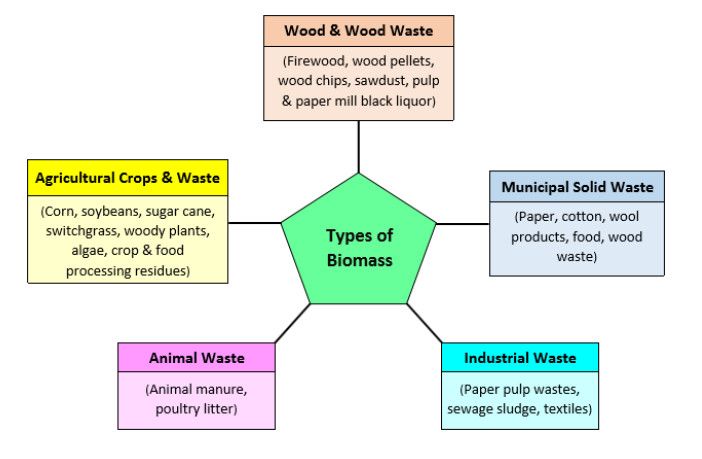


Figures(3) / Tables(8)

Eric Danso-Boateng, Osei-Wusu Achaw. Bioenergy and biofuel production from biomass using thermochemical conversions technologies—a review[J]. AIMS Energy, 2022, 10(4): 585-647. doi: 10.3934/energy.2022030


 DownLoad: