Adaptive PID sliding mode control based on new Quasi-sliding mode and radial basis function neural network for Omni-directional mobile robot

Thanh Tung Pham; Chi-Ngon Nguyen; Thanh Tung Pham; Chi-Ngon Nguyen

doi:10.3934/electreng.2023007

AIMS Electronics and Electrical Engineering

2023, Volume 7, Issue 2: 121-134. doi: 10.3934/electreng.2023007

Previous Article Next Article

Research article

Adaptive PID sliding mode control based on new Quasi-sliding mode and radial basis function neural network for Omni-directional mobile robot

Thanh Tung Pham ^{1
,
,},
Chi-Ngon Nguyen ²

1.
Vinh Long University of Technology Education, Vietnam
2.
Can Tho University, Vietnam

Received: 24 October 2022 Revised: 01 March 2023 Accepted: 10 March 2023 Published: 29 March 2023

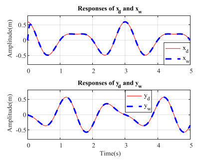
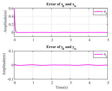
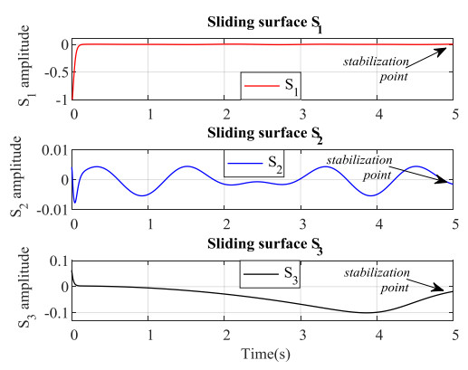
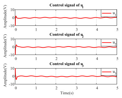
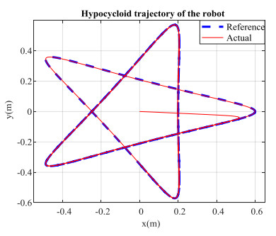
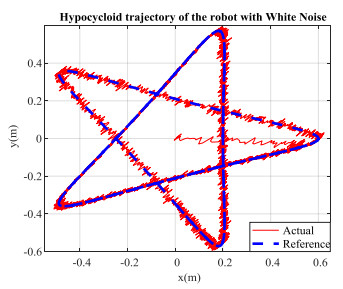
This article designs a PID sliding mode controller based on new Quasi-sliding mode (PID-SMC-NQ) and radial basis function neural network (RBFNN) for Omni-directional mobile robot. This is holonomic vehicles that can perform translational and rotational motions independently and simultaneously. The PID-SMC is designed to ensure that the robot's actual trajectory follows the desired in a finite time with the error converges to zero. To decrease chattering phenomena around the sliding surface, in the controller robust term, this paper uses the tanh (hyperbolic tangent) function, so called the new Quasi-sliding mode function, instead of the switch function. The RBFNN is used to approximate the nonlinear component in the PID-SMC-NQ controller. The RBFNN is considered as an adaptive controller. The weights of the network are trained online due to the feedback from output signals of the robot using the Gradient Descent algorithm. The stability of the system is proven by Lyapunov's theory. Simulation results in MATLAB/Simulink show the effectiveness of the proposed controller, the actual response of the robot converges to the reference with the rising time reaches 307.711 ms, 364.192 ms in the x-coordinate in the two-dimensional movement of the robot, the steady-state error is 0.0018 m and 0.00007 m, the overshoot is 0.13% and 0.1% in the y-coordinate, and the chattering phenomena is reduced.
- PID sliding mode control,
- new Quasi-sliding mode,
- radial basis function neural network,
- gradient descent,
- Omni-directional mobile robot,
- MATLAB/Simulink
Citation: Thanh Tung Pham, Chi-Ngon Nguyen. Adaptive PID sliding mode control based on new Quasi-sliding mode and radial basis function neural network for Omni-directional mobile robot[J]. AIMS Electronics and Electrical Engineering, 2023, 7(2): 121-134. doi: 10.3934/electreng.2023007

Related Papers:

Abstract

This article designs a PID sliding mode controller based on new Quasi-sliding mode (PID-SMC-NQ) and radial basis function neural network (RBFNN) for Omni-directional mobile robot. This is holonomic vehicles that can perform translational and rotational motions independently and simultaneously. The PID-SMC is designed to ensure that the robot's actual trajectory follows the desired in a finite time with the error converges to zero. To decrease chattering phenomena around the sliding surface, in the controller robust term, this paper uses the tanh (hyperbolic tangent) function, so called the new Quasi-sliding mode function, instead of the switch function. The RBFNN is used to approximate the nonlinear component in the PID-SMC-NQ controller. The RBFNN is considered as an adaptive controller. The weights of the network are trained online due to the feedback from output signals of the robot using the Gradient Descent algorithm. The stability of the system is proven by Lyapunov's theory. Simulation results in MATLAB/Simulink show the effectiveness of the proposed controller, the actual response of the robot converges to the reference with the rising time reaches 307.711 ms, 364.192 ms in the x-coordinate in the two-dimensional movement of the robot, the steady-state error is 0.0018 m and 0.00007 m, the overshoot is 0.13% and 0.1% in the y-coordinate, and the chattering phenomena is reduced.

References

[1]	Ren C, Li C, Hu L, Li X, Ma S (2022) Adaptive model predictive control for an omnidirectional mobile robot with friction compensation and incremental input constraints. T I Meas Control 44: 835–847. https://doi.org/10.1177/01423312211021321 doi: 10.1177/01423312211021321
[2]	Hacene N, Mendil B (2019) Motion Analysis and Control of Three-Wheeled Omnidirectional Mobile Robot. J Control Autom Electr Syst 30: 194–213. https://doi.org/10.1007/s40313-019-00439-0 doi: 10.1007/s40313-019-00439-0
[3]	Palacín J, Rubies E, Clotet E, Martínez D (2021) Evaluation of the Path-Tracking Accuracy of a Three-Wheeled Omnidirectional Mobile Robot Designed as a Personal Assistant. Sensors 21: 1–19. https://doi.org/10.3390/s21217216 doi: 10.1109/JSEN.2021.3109763
[4]	Kawtharani MA, Fakhari V, Haghjoo MR (2020) Tracking Control of an Omni-Directional Mobile Robot. International Congress on Human-Computer Interaction, Optimization and Robotic Applications (HORA), 1–8. https://doi.org/10.1109/HORA49412.2020.9152835 doi: 10.1109/HORA49412.2020.9152835
[5]	Andreev AS, Peregudova OA (2020) On Global Trajectory Tracking Control for an Omnidirectional Mobile Robot with a Displaced Center of Mass. Rus J Nonlin Dyn 16: 115–131. https://doi.org/10.20537/nd200110 doi: 10.20537/nd200110
[6]	Mou H (2020) Research On the Formation Method of Omnidirectional Mobile Robot Based On Dynamic Sliding Mode Control. Academic Journal of Manufacturing Engineering 18: 148–154.
[7]	Nganga-Kouya D, Okou F, Lauhic Ndong Mezui JM (2021) Modeling and Nonlinear Adaptive Control for Omnidirectional Mobile Robot. RJASET 18: 59–69. https://doi.org/10.19026/rjaset.18.6064 doi: 10.19026/rjaset.18.6064
[8]	Mehmood A, ul H. Shaikh I, Ali A (2021) Application of Deep Reinforcement Learning for Tracking Control of 3WD Omnidirectional Mobile Robot. ITC 50: 507–521. https://doi.org/10.5755/j01.itc.50.3.25979 doi: 10.5755/j01.itc.50.3.25979
[9]	Loucif F, Kechida S (2020) Optimization of sliding mode control with PID surface for robot manipulator by Evolutionary Algorithms. Open Computer Science 10: 396–407. https://doi.org/10.1515/comp-2020-0144 doi: 10.1515/comp-2020-0144
[10]	Liu J (2017) Sliding Mode Control Using MATLAB. Elsevier Science. https://doi.org/10.1016/B978-0-12-802575-8.00005-9 doi: 10.1016/B978-0-12-802575-8.00005-9
[11]	Li H, Huang S (2021) Research on the Prediction Method of Stock Price Based on RBF Neural Network Optimization Algorithm. E3S Web Conf 235: 1–5. https://doi.org/10.1051/e3sconf/202123503088 doi: 10.1051/e3sconf/202123503088
[12]	Wang H, Zhao Y, Pei J, Zeng D, Liu M (2019) Non-negative Radial Basis Function Neural Network in Polynomial Feature Space. J Phys Conf Ser 1168: 1–8. https://doi.org/10.1088/1742-6596/1168/6/062005 doi: 10.1088/1742-6596/1168/6/062005
[13]	Lemita A, Boulahbel S, Kahla S (2020) Gradient Descent Optimization Control of an Activated Sludge Process based on Radial Basis Function Neural Network. Eng Technol Appl Sci Res 10: 6080–6086. https://doi.org/10.48084/etasr.3714 doi: 10.48084/etasr.3714
[14]	Kaya AI, İLkuçar M, ÇiFci A (2019) Use of Radial Basis Function Neural Network in Estimating Wood Composite Materials According to Mechanical and Physical Properties. Erzincan Üniversitesi Fen Bilimleri Enstitüsü Dergisi 12: 116–123. https://doi.org/10.18185/erzifbed.428763 doi: 10.18185/erzifbed.428763
[15]	Lemita A, Boulahbel S, Kahla S, Sedraoui M (2020) Auto-Control Technique Using Gradient Method Based on Radial Basis Function Neural Networks to Control of an Activated Sludge Process of Wastewater Treatment. JESA 53: 671–679. https://doi.org/10.18280/jesa.530510 doi: 10.18280/jesa.530510
[16]	Pham TT, Le MT, Nguyen CN (2021) Omnidirectional Mobile Robot Trajectory Tracking Control with Diversity of Inputs. International Journal of Mechanical Engineering and Robotics Research 10: 639–644. https://doi.org/10.18178/ijmerr.10.11.639-644 doi: 10.18178/ijmerr.10.11.639-644
[17]	Mukherjee I, Routroy S (2012) Comparing the performance of neural networks developed by using Levenberg–Marquardt and Quasi-Newton with the gradient descent algorithm for modelling a multiple response grinding process. Expert Syst Appl 39: 2397–2407. https://doi.org/10.1016/j.eswa.2011.08.087 doi: 10.1016/j.eswa.2011.08.087

Reader Comments

Your name:*

Email:*
© 2023 the Author(s), licensee AIMS Press. This is an open access article distributed under the terms of the Creative Commons Attribution License (http://creativecommons.org/licenses/by/4.0)