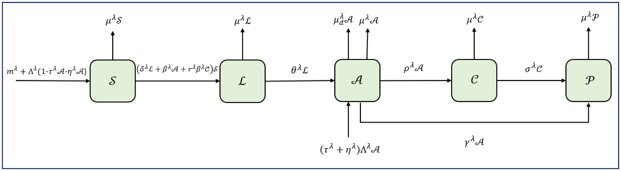
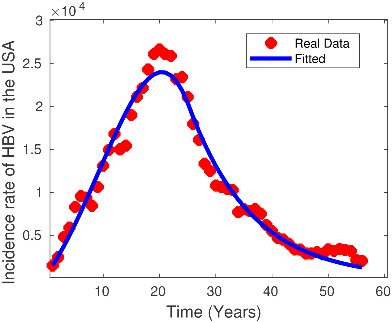
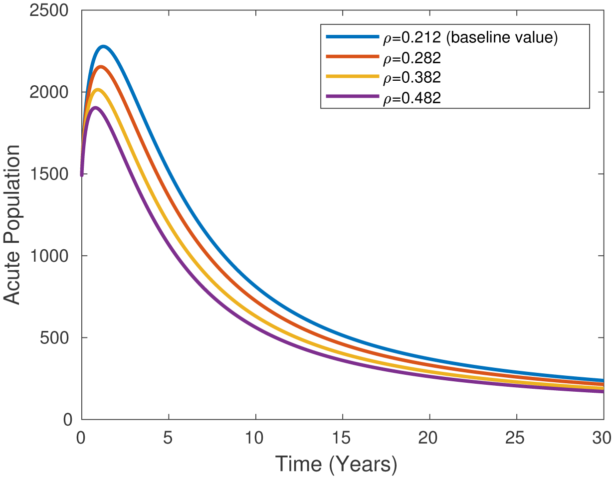
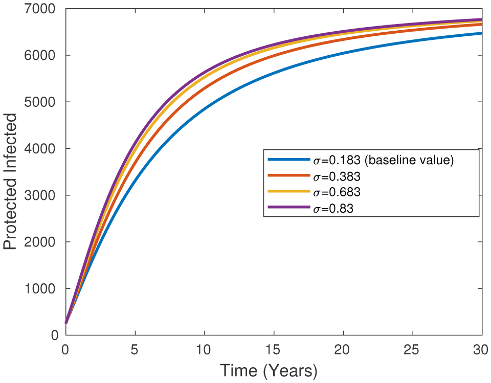
In this paper, a new mathematical model of Hepatitis B is studied to investigate the transmission dynamics of the Hepatitis B virus (HBV). Many diseases can start from the womb and find us humans throughout our lives. These diseases are specific abnormal conditions that negatively affect the structure or function of all or part of an organism and do not suddenly occur in any region due to external injury. In this study, we focus on HBV, and we state the graphics, interpretations, and detailed information about the disease and the newly established mathematical model of the disease. A fractional order differential equation system with a memory effect is used to model anomalous processes and to understand the effect of past infection events on the future spread dynamics of the system. In the model, susceptible, latent, acute, carrier, and recovered populations are taken into account by considering vertical transmission, which provides information about the inter-generational course of the disease. However, the migration effect is also used in the model due to the risk of disease transmission and increased migration in recent years. The course of the disease is examined using real data from the USA. Moreover, the model's positivity and boundedness are studied, and the equilibrium points are calculated. Additionally, the stability conditions for the disease-free equilibrium (DFE) are stated. A parameter calibration technique is used to determine the most accurate parameter values in the model. Finally, we provide numerical results and their biological interpretations to estimate the future course of the disease. The paper addresses the current migration problem with the migration parameter in the model. These differences from the literature can be regarded as important novelties of the paper.
Citation: Mehmet Yavuz, Kübra Akyüz, Naime Büşra Bayraktar, Feyza Nur Özdemir. Hepatitis-B disease modelling of fractional order and parameter calibration using real data from the USA[J]. AIMS Biophysics, 2024, 11(3): 378-402. doi: 10.3934/biophy.2024021
In this paper, a new mathematical model of Hepatitis B is studied to investigate the transmission dynamics of the Hepatitis B virus (HBV). Many diseases can start from the womb and find us humans throughout our lives. These diseases are specific abnormal conditions that negatively affect the structure or function of all or part of an organism and do not suddenly occur in any region due to external injury. In this study, we focus on HBV, and we state the graphics, interpretations, and detailed information about the disease and the newly established mathematical model of the disease. A fractional order differential equation system with a memory effect is used to model anomalous processes and to understand the effect of past infection events on the future spread dynamics of the system. In the model, susceptible, latent, acute, carrier, and recovered populations are taken into account by considering vertical transmission, which provides information about the inter-generational course of the disease. However, the migration effect is also used in the model due to the risk of disease transmission and increased migration in recent years. The course of the disease is examined using real data from the USA. Moreover, the model's positivity and boundedness are studied, and the equilibrium points are calculated. Additionally, the stability conditions for the disease-free equilibrium (DFE) are stated. A parameter calibration technique is used to determine the most accurate parameter values in the model. Finally, we provide numerical results and their biological interpretations to estimate the future course of the disease. The paper addresses the current migration problem with the migration parameter in the model. These differences from the literature can be regarded as important novelties of the paper.

| [1] | Medical Park Hastaneler Grubu, 2021. Available from: https://www.medicalpark.com.tr/bulasici-hastaliklar/hg-2134 |
| [2] |
Sorrell MF, Belongia EA, Costa J, et al. (2009) National institutes of health consensus development conference statement: management of hepatitis B. Ann Intern Med 150: 104-110. https://doi.org/10.7326/0003-4819-150-2-200901200-00100 
|
| [3] |
Kaya A, Erbey MF, Okur M, et al. (2011) Hepatitis B virus seropositivity and vaccination for children aged 0-18 in the Van region/Van yoresinde 0-18 yaslan arasindaki cocuklarda hepatit B virusu seropozitifligi ve asilanma durumu. J Pediatr Inf 5: 132-136. https://doi.org/10.5152/ced.2011.46
|
| [4] |
Hsu HY, Chang MH, Chen DS, et al. (1986) Baseline seroepidemiology of hepatitis B virus infection in children in Taipei, 1984: a study just before mass hepatitis B vaccination program in Taiwan. J Med Virol 18: 301-307. https://doi.org/10.1002/jmv.1890180402
|
| [5] |
Chang MH, Chen CJ, Lai MS, et al. (1997) Universal hepatitis B vaccination in Taiwan and the incidence of hepatocellular carcinoma in children. New Engl J Med 336: 1855-1859. https://doi.org/10.1056/NEJM199706263362602
|
| [6] | Demir A, Kansu Tanca A (2023) Kronik hepatit B virüs enfeksiyonunda antiviral tedavi yönetimi. Çocukluk Çağında Her Yönüyle Hepatit B Virüs Enfeksiyonu . Ankara: Türkiye Klinikleri Yayınevi 45-49. |
| [7] |
Hethcote HW (2000) The mathematics of infectious diseases. SIAM Rev 42: 599-653. https://doi.org/10.1137/S0036144500371907
|
| [8] | Işık N, Kaya A (2020) İnfeksiyöz Hastalıkların Yayılması ve Kontrolünde Matematiksel Modeller ve Sürü Bağışıklama. Atatürk Üniversitesi Vet Bil Derg 15: 301-307. http://dx.doi.org/10.17094/ataunivbd.715371 |
| [9] | Kermack WO, McKendrick AG (1927) A contribution to the mathematical theory of epidemics. Proceedings of the Royal Society of London, Series A, Containing Papers of a Mathematical and Physical Character 115: 700-721. https://doi.org/10.1098/rspa.1927.0118 |
| [10] | Kamyad AV, Akbari R, Heydari AA (2014) Mathematical modeling of transmission dynamics and optimal control of vaccination and treatment for hepatitis B virus. Comput Math Method M 2014: 475451. https://doi.org/10.1155/2014/475451 |
| [11] |
Ciupe SM, Hews S (2012) Mathematical models of e-antigen mediated immune tolerance and activation following prenatal HBV infection. PLoS One 7: e39591. https://doi.org/10.1371/journal.pone.0039591
|
| [12] |
Guedj J, Rotman Y, Cotler SJ, et al. (2014) Understanding early serum hepatitis D virus and hepatitis B surface antigen kinetics during pegylated interferon-alpha therapy via mathematical modeling. Hepatology 60: 1902-1910. https://doi.org/10.1002/hep.27357
|
| [13] | Wodajo FA, Mekonnen TT (2022) Effect of intervention of vaccination and treatment on the transmission dynamics of HBV disease: a mathematical model analysis. J Math 9968832. https://doi.org/10.1155/2022/9968832 |
| [14] |
Goyal A, Ribeiro RM, Perelson AS (2017) The role of infected cell proliferation in the clearance of acute HBV infection in humans. Viruses 9: 350. https://doi.org/10.3390/v9110350
|
| [15] |
Carracedo Rodriguez A, Chung M, Ciupe SM (2017) Understanding the complex patterns observed during hepatitis B virus therapy. Viruses 9: 117. https://doi.org/10.3390/v9050117
|
| [16] |
Ciupe SM (2018) Modeling the dynamics of hepatitis B infection, immunity, and drug therapy. Immunol Rev 285: 38-54. https://doi.org/10.1111/imr.12686
|
| [17] |
Dahari H, Shudo E, Ribeiro RM, et al. (2009) Modeling complex decay profiles of hepatitis B virus during antiviral therapy. Hepatology 49: 32-38. https://doi.org/10.1002/hep.22586
|
| [18] |
Goyal A, Murray JM (2016) Modelling the impact of cell-to-cell transmission in hepatitis B virus. PLoS One 11: e0161978. https://doi.org/10.1371/journal.pone.0161978
|
| [19] |
Colombatto P, Civitano L, Bizzarri R, et al. (2006) A multiphase model of the dynamics of HBV infection in HBeAg-negative patients during pegylated interferon-α2a, lamivudine and combination therapy. Antivir Ther 11: 197-212. https://doi.org/10.1177/135965350601100201
|
| [20] |
Cangelosi Q, Means SA, Ho H (2017) A multi-scale spatial model of hepatitis-B viral dynamics. PLoS One 12: e0188209. https://doi.org/10.1371/journal.pone.0188209
|
| [21] | Khan MA, Islam S, Arif M, et al. (2013) Transmission model of hepatitis B virus with the migration effect. BioMed Res Int 2013: 150681. https://doi.org/10.1155/2013/150681 |
| [22] | Din A, Abidin MZ (2022) Analysis of fractional-order vaccinated Hepatitis-B epidemic model with Mittag-Leffler kernels. Math Model Num Simul Appl 2: 59-72. https://doi.org/10.53391/mmnsa.2022.006 |
| [23] |
Yavuz M, Özköse F, Susam M, et al. (2023) A new modeling of fractional-order and sensitivity analysis for hepatitis-b disease with real data. Fractal Fract 7: 165. https://doi.org/10.3390/fractalfract7020165
|
| [24] | Mustapha UT, Ahmad YU, Yusuf A, et al. (2023) Transmission dynamics of an age-structured Hepatitis-B infection with differential infectivity. Bull Biomath 1: 124-152. https://doi.org/10.59292/bulletinbiomath.2023007 |
| [25] |
Wodajo FA, Gebru DM, Alemneh HT (2023) Mathematical model analysis of effective intervention strategies on transmission dynamics of hepatitis B virus. Sci Rep 13: 8737. https://doi.org/10.1038/s41598-023-35815-z
|
| [26] |
Xu C, Wang Y, Cheng K, et al. (2023) A mathematical model to study the potential hepatitis B virus infections and effects of vaccination strategies in China. Vaccines 11: 1530. https://doi.org/10.3390/vaccines11101530
|
| [27] |
Khatun Z, Islam MS, Ghosh U (2020) Mathematical modeling of hepatitis B virus infection incorporating immune responses. Sens Int 1: 100017. https://doi.org/10.1016/j.sintl.2020.100017
|
| [28] |
Aniji M, Kavitha N, Balamuralitharan S (2020) Mathematical modeling of hepatitis B virus infection for antiviral therapy using LHAM. Adv Differ Equ 2020: 408. https://doi.org/10.1186/s13662-020-02770-2
|
| [29] |
Endashaw EE, Mekonnen TT (2022) Modeling the effect of vaccination and treatment on the transmission dynamics of hepatitis B virus and HIV/AIDS coinfection. J Appl Math 2022: 5246762. https://doi.org/10.1155/2022/5246762
|
| [30] | Khan M, Khan T, Ahmad I, et al. (2022) Modeling of hepatitis B virus transmission with fractional analysis. Math Probl Eng 2022: 6202049. https://doi.org/10.1155/2022/6202049 |
| [31] |
Khan T, Jung IH, Zaman G (2019) A stochastic model for the transmission dynamics of hepatitis B virus. J Biol Dynam 13: 328-344. https://doi.org/10.1080/17513758.2019.1600750
|
| [32] |
Zhao S, Xu Z, Lu Y (2000) A mathematical model of hepatitis B virus transmission and its application for vaccination strategy in China. Int J Epidemiol 29: 744-752. https://doi.org/10.1093/ije/29.4.744
|
| [33] |
Danane J, Allali K, Hammouch Z (2020) Mathematical analysis of a fractional differential model of HBV infection with antibody immune response. Chaos Soliton Fract 136: 109787. https://doi.org/10.1016/j.chaos.2020.109787
|
| [34] |
Goldstein ST, Zhou F, Hadler SC, et al. (2005) A mathematical model to estimate global hepatitis B disease burden and vaccination impact. Int J Epidemiol 34: 1329-1339. https://doi.org/10.1093/ije/dyi206
|
| [35] |
Liang P, Zu J, Zhuang G (2018) A literature review of mathematical models of hepatitis B virus transmission applied to immunization strategies from 1994 to 2015. J Epidemiol 28: 221-229. https://doi.org/10.2188/jea.je20160203
|
| [36] |
Li M, Zu J (2019) The review of differential equation models of HBV infection dynamics. J Virol Methods 266: 103-113. https://doi.org/10.1016/j.jviromet.2019.01.014
|
| [37] | Min L, Su Y, Kuang Y (2008) Mathematical analysis of a basic virus infection model with application to HBV infection. Rocky Mt J Math 38: 1573-1585. https://doi.org/10.1216/RMJ-2008-38-5-1573 |
| [38] |
Goyal A, Liao LE, Perelson AS (2019) Within-host mathematical models of hepatitis B virus infection: Past, present, and future. Curr Opin Syst Biol 18: 27-35. https://doi.org/10.1016/j.coisb.2019.10.003
|
| [39] |
Zhang S, Zhou Y (2012) The analysis and application of an HBV model. Appl Math Model 36: 1302-1312. https://doi.org/10.1016/j.apm.2011.07.087
|
| [40] |
Naik PA, Yavuz M, Qureshi S, et al. (2024) Memory impacts in hepatitis C: a global analysis of a fractional-order model with an effective treatment. Comput Method Prog Biomed 254: 108306. https://doi.org/10.1016/j.cmpb.2024.108306
|
| [41] |
Mustapha UT, Maigoro YA, Yusuf A, et al. (2024) Mathematical modeling for the transmission dynamics of cholera with an optimal control strategy. Bull Biomath 2: 1-20. https://doi.org/10.59292/bulletinbiomath.2024001
|
| [42] | Kumar P, Erturk VS (2021) Dynamics of cholera disease by using two recent fractional numerical methods. Math Model Numer Simul Appl 1: 102-111. https://doi.org/10.53391/mmnsa.2021.01.010 |
| [43] | Ahmed I, Akgül A, Jarad F, et al. (2023) A Caputo-Fabrizio fractional-order cholera model and its sensitivity analysis. Math Model Numer Simul Appl 3: 170-187. http://dx.doi.org/10.53391/mmnsa.1293162 |
| [44] | Bolaji B, Onoja T, Agbata C, et al. (2024) Dynamical analysis of HIV-TB co-infection transmission model in the presence of treatment for TB. Bull Biomath 2: 21-56. https://doi.org/10.59292/bulletinbiomath.2024002 |
| [45] | Evirgen F, Uçar E, Uçar S, et al. (2023) Modelling influenza a disease dynamics under Caputo-Fabrizio fractional derivative with distinct contact rates. Math Model Numer Simul Appl 3: 58-73. https://doi.org/10.53391/mmnsa.1274004 |
| [46] |
Duru EC, Anyanwu MC (2023) Mathematical model for the transmission of mumps and its optimal control. Biometrical Lett 60: 77-95. http://dx.doi.org/10.2478/bile-2023-0006
|
| [47] |
Raeisi E, Yavuz M, Khosravifarsani M, et al. (2024) Mathematical modeling of interactions between colon cancer and immune system with a deep learning algorithm. Eur Phys J Plus 139: 345. https://doi.org/10.1140/epjp/s13360-024-05111-4
|
| [48] | Salih RI, Jawad S, Dehingia K, et al. (2024) The effect of a psychological scare on the dynamics of the tumor-immune interaction with optimal control strategy. Int J Optim Control The Appl 14: 276-293. https://doi.org/10.11121/ijocta.1520 |
| [49] | Joshi H, Yavuz M, Özdemir N (2024) Analysis of novel fractional order plastic waste model and its effects on air pollution with treatment mechanism. J Appl Anal Comput 14: 3078-3098. https://doi.org/10.11948/20230453 |
| [50] |
Joshi H, Yavuz M (2024) Numerical analysis of compound biochemical calcium oscillations process in hepatocyte cells. Adv Biol 8: 2300647. https://doi.org/10.1002/adbi.202300647
|
| [51] | Munson A (2023) A harmonic oscillator model of atmospheric dynamics using the Newton-Kepler planetary approach. Math Model Numer Simul Appl 3: 216-233. https://doi.org/10.53391/mmnsa.1332893 |
| [52] | Xu C, Farman M, Shehzad A (2023) Analysis and chaotic behavior of a fish farming model with singular and non-singular kernel. Int J Biomath 2350105. https://doi.org/10.1142/S179352452350105X |
| [53] | Yapışkan D, Eroğlu BBİ (2024) Fractional-order brucellosis transmission model between interspecies with a saturated incidence rate. Bull Biomath 2: 114-132. https://doi.org/10.59292/bulletinbiomath.2024005 |
| [54] | Naik PA, Eskandari Z, Yavuz M, et al. (2024) Bifurcation results and chaos in a two-dimensional predator-prey model incorporating Holling-type response function on the predator. Discrete Cont Dyn S . https://doi.org/10.3934/dcdss.2024045 |
| [55] | Ghosh D, Santra PK, Mahapatra GS (2023) A three-component prey-predator system with interval number. Math Model Numer Simul Appl 3: 1-16. https://doi.org/10.53391/mmnsa.1273908 |
| [56] |
Wiratsudakul A, Suparit P, Modchang C (2018) Dynamics of Zika virus outbreaks: an overview of mathematical modeling approaches. PeerJ 6: e4526. https://doi.org/10.7717/peerj.4526
|
| [57] |
Möhler L, Flockerzi D, Sann H, et al. (2005) Mathematical model of influenza A virus production in large-scale microcarrier culture. Biotechnol Bioeng 90: 46-58. https://doi.org/10.1002/bit.20363
|
| [58] | Podlubny I (1999) Fractional Differential Equations. Academic Press. |
| [59] |
Lin W (2007) Global existence theory and chaos control of fractional differential equations. J Math Anal Appl 332: 709-726. https://doi.org/10.1016/j.jmaa.2006.10.040
|
| [60] |
Naik PA, Yavuz M, Qureshi S, et al. (2020) Modeling and analysis of COVID-19 epidemics with treatment in fractional derivatives using real data from Pakistan. Eur Phys J Plus 135: 795. https://doi.org/10.1140/epjp/s13360-020-00819-5
|
| [61] |
Driessche P, Watmough J (2002) Reproduction numbers, and sub-threshold endemic equilibria for compartmental models of disease transmission. Math Biosci 180: 29-48. https://doi.org/10.1016/S0025-5564(02)00108-6
|
| [62] |
Ahmed E, Elgazzar AS (2007) On fractional order differential equations model for nonlocal epidemics. Physica A 379: 607-614. https://doi.org/10.1016/j.physa.2007.01.010
|
| [63] | Matignon D Stability results for fractional differential equations with applications to control processing (1996)2: 963-968. |
| [64] |
Danane J, Yavuz M, Yıldız M (2023) Stochastic modeling of three-species prey-predator model driven by Lévy jump with mixed holling-II and Beddington-DeAngelis functional responses. Fractal Fract 7: 751. https://doi.org/10.3390/fractalfract7100751
|
| [65] |
Yavuz M, ur Rahman M, Yildiz M, et al. (2024) Mathematical modeling of middle east respiratory syndrome corona virus with bifurcation analysis. Contem Math 5: 3997-4012. https://doi.org/10.37256/cm.5320245004
|
| [66] | Eskandari Z, Naik PA, Yavuz M (2024) Dynamical behaviors of a discrete-time prey-predator model with harvesting effect on the predator. J Appl Anal Comput 14: 283-297. https://doi.org/10.11948/20230212 |
| [67] | Statistics on deaths and causes of death, 2021. Available from: https://data.tuik.gov.tr/Bulten/Index?p=Olum-ve-Olum-Nedeni-Istatistikleri-2021-45715# |
| [68] |
Garrappa R (2010) On linear stability of predictor-corrector algorithms for fractional differential equations. Int J Comput Math 87: 2281-2290. https://doi.org/10.1080/00207160802624331
|
| [69] |
Garrappa R (2018) Numerical solution of fractional differential equations: a survey and a software tutorial. Mathematics 6: 16. https://doi.org/10.3390/math6020016
|
| [70] | Binbay NE, Gümgüm HB (2019) Bloch denklemlerinin, nümerik yöntemlerle çözümü 155-184. |
| [71] | Samko SG, Kilbas AA, Marichev OI (1993) Fractional integrals and derivatives. Theory and Applications . Langhorne: Gordon and Breach Science Publishers. |
| [72] | Surveillance for Viral Hepatitis - United States, 2015. Available from: https://www.cdc.gov/hepatitis/statistics/2015surveillance/index.htm#tabs-5-3 |
Figures(9) / Tables(1)

Mehmet Yavuz, Kübra Akyüz, Naime Büşra Bayraktar, Feyza Nur Özdemir. Hepatitis-B disease modelling of fractional order and parameter calibration using real data from the USA[J]. AIMS Biophysics, 2024, 11(3): 378-402. doi: 10.3934/biophy.2024021


 DownLoad: