Design of an iterative method for enhanced early prediction of acute coronary syndrome using XAI analysis

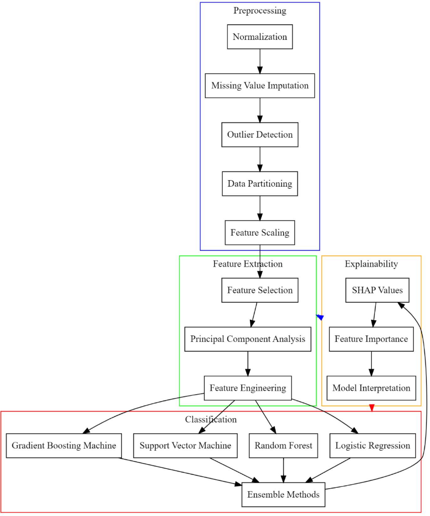
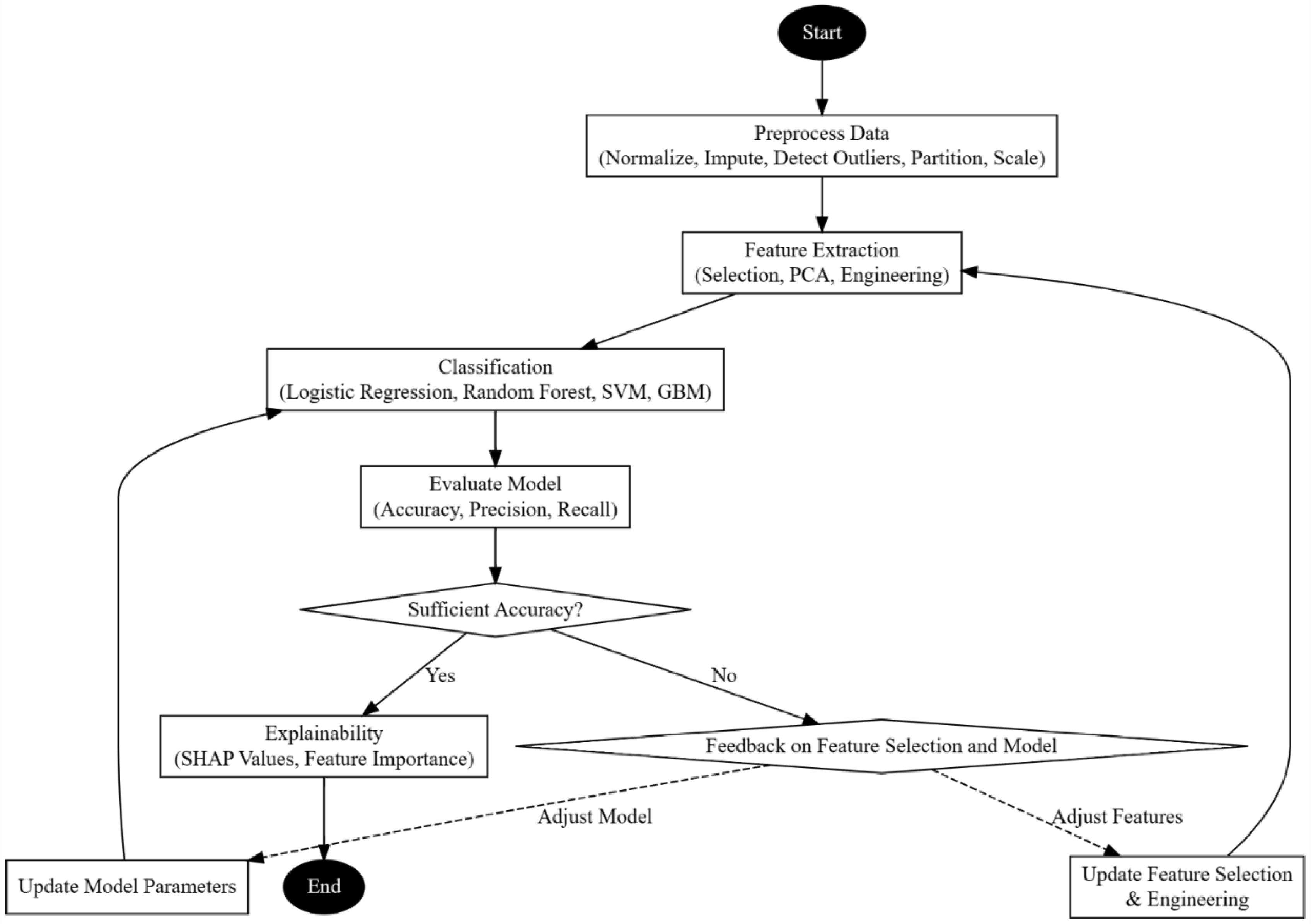
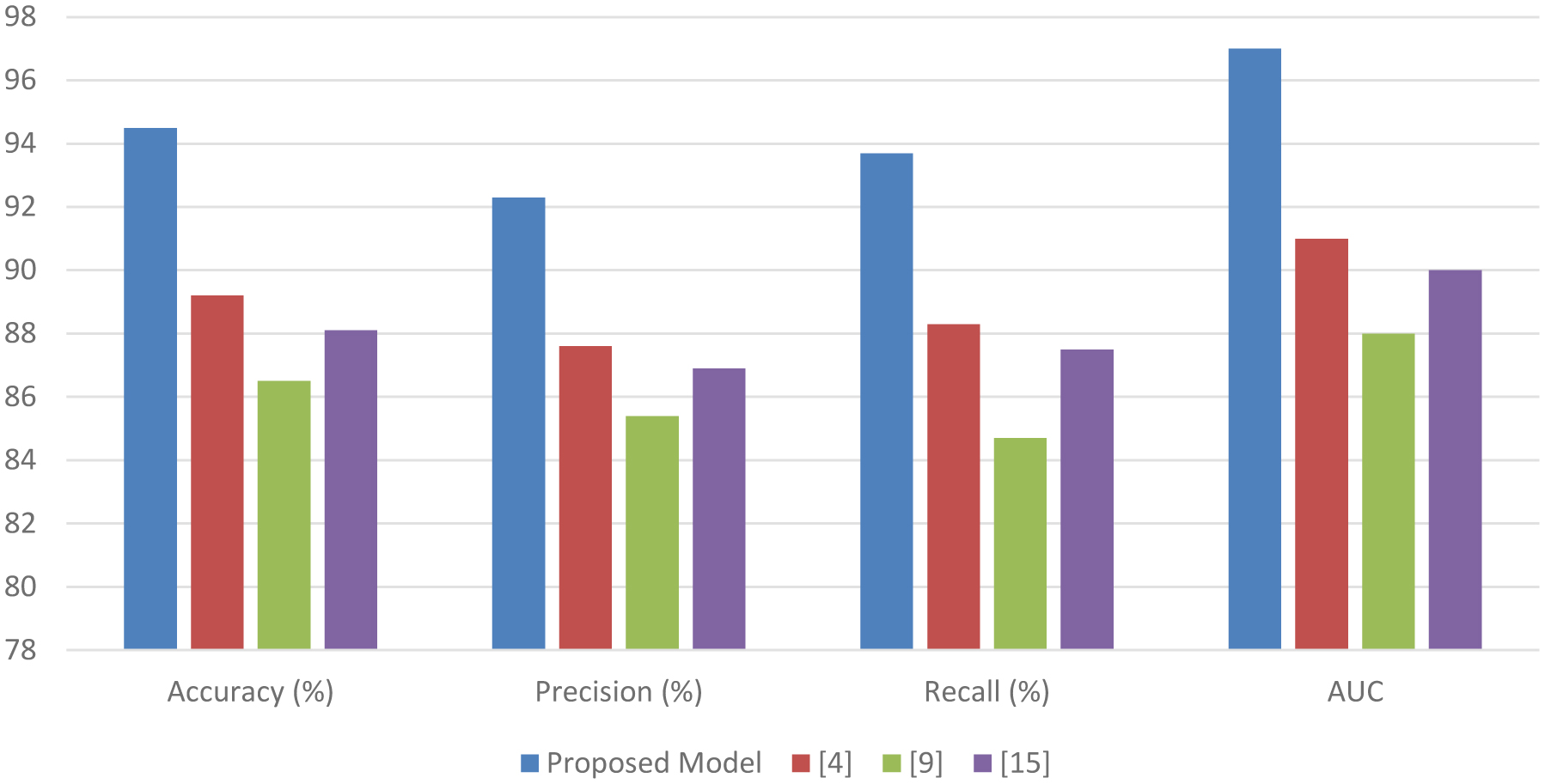
1.   Introduction

The inception of heart diseases as the principal cause of mortality globally necessitates the advancement of diagnostic methodologies, particularly for Acute Coronary Syndrome (ACS), which is a critical subset associated with high mortality rates. ACS represents a spectrum of conditions attributable to the diminution of blood flow to the coronary arteries, including myocardial infarction with ST-segment elevation, myocardial infarction without ST-segment elevation, and unstable angina. The latent and unpredictable nature of ACS underscores the imperative for early prediction and intervention to mitigate adverse outcomes.

Traditionally, ACS prediction has been predicated on clinical evaluations and conventional risk factor assessments. However, these methods often fall short in their predictive accuracy and timeliness, constrained by the static nature of the risk factors and the inability to capture complex interactions among them. The advent of machine learning (ML) in healthcare introduces a novel approach, offering dynamic, non-linear analytical capabilities that transcend traditional statistical approaches.

Despite the ability of artificial intelligence to enhance the predictive models, the application in ACS prediction confronts challenges such as imbalanced datasets, missing values, and the high dimensionality of clinical data. Addressing these challenges necessitates a meticulous approach to data preprocessing and feature selection, thus ensuring the integrity and relevance of the data fed into predictive algorithms.

This paper delineates an iterative method for ACS prediction, thereby integrating advanced ML algorithms with robust data preprocessing and feature selection techniques. The proposed framework aims to refine the predictive accuracy by addressing the intrinsic challenges of clinical datasets. By employing algorithms such as Gradient Boosting, Deep Forest, Support Vector Machines, and Logistic Regression, the study traverses beyond conventional predictive paradigms, optimizing for sensitivity, specificity, and timeliness—critical metrics in ACS prognosis.

Moreover, the research emphasizes the interpretability of ML models in clinical settings, which is an aspect paramount for patient care and medical decision-making. Through the analysis of logistic regression coefficients and SHapley Additive exPlanations (SHAP) values, the study elucidates the contribution of individual risk factors. Moreover, by adding a correlation analysis with a recursive feature removal, the important features are extracted, thus improving the Accountability and efficiency of the model.

2.   Materials and methods

2.1.   In-depth review of existing models

The incessant evolution of ML and data science within the healthcare sector has markedly shifted the paradigms of disease prediction, diagnosis, and prevention. ACS, which is a critical condition with significant morbidity and mortality rates, has been at the forefront of this shift. Recent research endeavors, as evidenced by studies in Table 1, underscored a collective move towards integrating advanced computational techniques to enhance ACS diagnostics and secondary prevention measures. The methodologies employed across these studies range from ensemble ML to data science analysis, each aiming to surmount the limitations inherent in traditional diagnostic approaches.

Upon meticulous examination of the recent literature spanning various methodologies and findings in ACS and cardiovascular disease prediction, several thematic insights emerge. First, the deployment of ensemble ML and stacking ensemble models, as seen in studies [2] and [4], reflects an effective strategy to overcome the challenges posed by imbalanced datasets, which are prevalent in healthcare data. These methods have been shown to improve the robustness and accuracy of the predictive models, thereby enhancing their clinical applicability. Second, the utilization of data science techniques for secondary prevention, as delineated in studies [3] and [5], underscores the growing emphasis on preventive healthcare. By analyzing patient profiles and historical data, these approaches enable the identification of at-risk individuals, thereby facilitating early intervention and tailored treatment strategies.

However, the analysis also unveils a recurrent theme of limitations across the studies. A common constraint is the lack of extensive validation across diverse and larger patient cohorts, which raises questions regarding the scalability and adaptability of these models to different demographic and clinical settings. Moreover, while the push towards advanced algorithms and computational models is evident, there remains a critical need to enhance the interpretability and transparency of these models to ensure their seamless integration into clinical practice.

2.2.   Design of the proposed model for ACS analysis

In the domain of biomedical signal processing, data integrity is paramount, particularly within the context of ACS detection. The initial phase of the methodology is the meticulous design of data preprocessing strategies aimed at refining the collected Electrocardiogram (ECG) and Echocardiogram (Echo) samples. The primary goal is to transform the raw datasets into a reliable format conducive to the application of sophisticated ML models. The initial step involves the normalization of the ECG and Echo datasets, where each sample xi in the dataset is transformed via Eq 1:

where µ is the mean and σ represents the standard deviation of the dataset, respectively. This standardization ensures that the dataset has a zero mean with a standard deviation of one, which mitigates discrepancies caused by varying scales and amplitudes inherent in raw biomedical signals. Following normalization, the methodology employs advanced missing value imputation to address gaps in the data, which is a common issue with real-world biomedical datasets and samples.

Given a set of observed values O and missing values M, the imputation process is represented via Eq 2:

where N represents the total number of observed data samples, ε represents the error term, and F represents Iterative Expectation Maximization, which iteratively includes the following two steps: the model parameters are updated using the full data in the M-Step, which are now filled in with estimated missing values based on the data patterns, and the value gaps are estimated using the current assessment of the model parameters in the E-step. This process is mathematically encapsulated using an iterative set of operations, represented via Eqs 3 and 4 as follows:

where the parameters of the predictive model are given as θ, and the likelihood function for this process is represented by L. Next, as per Figure 1, outlier detection follows, which involves the identification and handling of aberrant values that significantly deviate from the norm, as these can skew the analysis. This work uses Z-scores, where outliers are detected via Eq 5:

where values of Z that exceed a threshold, typically 3 (corresponding to three standard deviations for this process), are flagged as outliers. However, in the context of ECG and Echo data, more sophisticated techniques such as the interquartile range (IQR) are employed, in which the outliers are identified as values that fall below Q1−1.5×IQR or above Q3+1.5×IQR, where Q1 and Q3 are the first and third quartiles, respectively. Subsequent to the detection and mitigation of the outliers, the data undergoes a transformation phase aimed at enhancing the model's interpretability and predictive performance. This includes the application of a principal component analysis (PCA), where the transformation T = XW is applied, X represents the data matrix, and W represents the matrix of eigenvectors obtained from the covariance matrix of X samples. This reduces the dimensionality while preserving the variance, and is distilled into fewer, more significant components in the process.

Finally, the integrity and reliability of the pre-processed ECG and Echo samples are ensured through a comprehensive anomaly detection scheme, typically employing autoencoders in the context of neural networks. The reconstruction error is ε=|x−x′|, where x′ is the reconstructed input after compression, and decompression through the autoencoder is calculated in this process. Samples with a reconstruction error that exceed a specified threshold are flagged for review, which indicate potential anomalies or novel patterns that are not captured during the initial data cleaning phase.

As per Figure 2, within the framework of predictive modeling, feature selection emerges as a critical step for this process, particularly for ACS prediction from pre-processed biomedical datasets. This step aims to distill the most informative predictive indicators from extensive clinical datasets, thereby enhancing the model performance and interpretability while reducing the computational complexity levels. The recursive feature elimination (RFE) process commences with the establishment of an initial model, using an SVM, which assigns weights to features based on their importance in predicting the target variable sets. Representing the weight vector from the SVM or coefficients from Logistic Regression as w, the importance of each feature fi is quantified as |wi|, with larger values indicating greater importance levels.

The RFE algorithm iteratively refines the feature set. Initially, it considers all features, which are represented by the set F = {f₁, f₂, ..., f_n}, where n is the total number of features. In each iteration, the algorithm performs the following steps: first, the model is trained on the current set of features and the importance of each feature is calculated by this process; and second, the feature with the smallest |wi| (deemed the least important) is removed, formally represented via Eq 6:

where f_min is the feature corresponding to the smallest |wi| sets. This process iteratively continues, eliminating one feature per iteration, either until a predefined number of features remain or until the model performance meets a specified criterion process.

Concurrently, a correlation analysis serves as a supplementary mechanism to scrutinize the interdependencies among features. The Pearson correlation coefficient, represented as ρxy, quantifies the linear relationship between the two features x and y, calculated via Eq 7:

where x and y are the mean values of features x and y, respectively. Features exhibiting high correlation coefficients (either positive or negative) indicate redundancy, as they provide overlapping information, which could lead to multicollinearity in predictive models. In the context of ACS prediction, the correlation threshold θ is predetermined, and pairs of features that exceed this threshold are flagged. The process involves examining all possible pairs of remaining features, represented by the set P={(fa,fb)|fa,fb∈F,a≠b}, and identifying e pairs where ρfafb|>θ by the process. For each identified pair, the feature with the lesser importance based on the previously established metric |wi| is earmarked for elimination operations.

The synthesis of RFE and the correlation analysis cultivates a robust feature selection strategy, iteratively pruning and evaluating features to only retain those with significant predictive power and a minimal redundancy. This iterative elimination and evaluation are mathematically encapsulated through the update equations for the feature sets and the calculation of the feature importances and correlations, which adhere to the objective of optimizing the predictive capability of the model while maintaining parsimony in the feature space. The culmination of this process yields a refined set of features, ‘F’, which encompasses the most critical predictive indicators, thereby facilitating the construction of a more accurate and interpretable model for early detection of ACD from pre-processed ECG and Echo samples.

Next, as per Figure 2, in the analytical framework underpinning the study on ACS detection, a sophisticated ensemble of ML algorithms is employed, each tailored to the nuanced requirements of biomedical signal classification operations. The methodology integrates Logistic Regression, Deep Forest, SVMs, and Gradient Boosting Machines (GBMs), which are crafted to balance computational rigor with interpretative clarity, thereby optimizing the spectrum of performance metrics. Beginning with the Logistic Regression, which is a cornerstone of statistical classification models, it is predicated on the logistic function to model the probability that a given input belongs to a particular category of ACS. For a set of features x = [x₁, x₂, ..., x_n] and corresponding coefficients β = [β₀, β₁, ..., β_n], the probability of the positive class P (Y = 1|x) is given by the sigmoid process represented via Eq 8:

where z=β0+β1x1+...+βnxn, and the model parameters β are estimated through maximum likelihood estimation, which optimizes the cost function represented via Eq 9:

where y_i is the class label for the i-th sample sets and m is the number of training examples. On the other hand, during the training phase, the Deep Forest method builds a large number of decision trees and outputs the class that is the mean of the classes of each of the trees. The forecast for a new sample x in a Deep Forest with N trees is generated by adding the predictions from each individual tree. Eq 10 represents the categorization function:

where Ti represents the i-th decision trees. The diversity among the trees, which is essential for the model's robustness, is ensured through the random selection of features and bootstrapping of the training samples. Furthermore, the SVM offers a powerful and versatile modeling technique and is especially efficacious in high-dimensional spaces. In its basic form, SVM looks for the hyperplane in feature spaces that best divides the classes. Eq 11 defines the choice function:

where the normal vector to the hyperplane is given as w, and b represents the bias. The optimal hyperplane maximizes the margin between the two classes, which is formulated as a convex optimization task and is represented via Eq 12:

In nonlinear cases, the kernel operation is applied, which transforms the input space into a higher-dimensional space, where a linear separator is found using the radial basis function (RBF), and is represented via Eq 13:

Lastly, GBMs operate by consecutively adding predictors to an ensemble, each correcting its predecessors. This method involves the construction of decision trees one at a time, where each new tree helps to correct errors made by previously trained trees. Given a loss function L(y,F(x)), the addition of a new tree aims to minimize L by fitting the negative gradient of the loss function, which effectively performs a gradient descent in the function space. The update rule for the ensemble model at the n-th step is expressed via Eq 14:

where hn(x) is the n-th decision tree, and ρn is the step size, which is determined through line search to minimize the loss. These methods are fused to obtain the final class, which is then explained using a SHAP analysis. This analysis assists Doctors and Technicians to estimate root cause of ACS. The interpretative insights into the risk factor significance are garnered by assimilating the logistic regression coefficients with SHAP values in this process. The fusion delineates a robust framework for personalized patient risk assessments, which underpins the intricate dynamics between the clinical features and the ACS risk predictions.

At its core, a logistic regression employs a logistic function to estimate the probabilities that particular instances fall into one of two classes for this process. For an instance with features x = [x₁, x₂, ..., x_n], the logistic regression model predicts the probability of the instance being a member of the class using the logistic function represented via Eq 15:

where β₀, β₁, ..., β_n represent the regression coefficients that correspond to the intercept and features, respectively. These coefficients are derived through the optimization of the likelihood function, where a gradient ascent is used and encapsulated by the update rule represented via Eq 16:

where α is the learning rate, m is the number of samples, andσrepresents the logistic based classification process. Upon the establishment of the logistic regression model, the interpretability is significantly enhanced through the application of SHAP values, which provide a measure of the impact of each feature on the prediction outcome. The foundation of the SHAP values lies in cooperative game theory, particularly in the Shapley value, which fairly distributes “payouts” (in this case, contributions to the prediction) among the players (features). For a given feature value, the SHAP value is calculated through an iterative process, and compares predictions with and without the feature across all possible combinations of other features. Mathematically, for a feature j and a prediction instance x, the SHAP value is given via Eq 17:

where N is the set of all features, S is a subset of features that exclude j, and fx(S) represents the prediction when only the features in S are considered by the process. This calculation involves assessing the marginal contribution of the feature j over all possible feature subsets, which is a computationally intensive task that is approximated in practical use case scenarios. Integrating SHAP values into the logistic regression framework allows for the decomposition of the prediction into contributions from each feature. For a binary classification problem such as ACS detection, the SHAP value for a feature in relation to a specific prediction can significantly elucidate the directional influence (positive or negative) of the feature on the log odds of the predicted outcome. In terms of log odds, the overall model output is expressed as the sum of all the feature SHAP values plus a base value (the model output when no features are present) via Eq 18:

where p is the predicted probability of ACS presence in the process. The exhaustive computation of the SHAP values alongside the logistic regression coefficients furnishes a transparent and detailed canvas which illustrates how each clinical feature influences the risk prediction of ACS. During this setting, a lack of transparency may result; to avoid this problem, the study integrates SHAP values, which provide a unified framework to interpret the outputs of various ML models, including complex ones such as GBM and Deep Forest. SHAP values, which are derived from cooperative game theory, quantify the contribution of each feature to the model's prediction, thus offering a clear explanation of how different clinical variables influence the outcome. A result analysis of this model was performed by comparing its performance with existing methods in the next section of this text.

3.   Result analysis

In the construction of the experimental setup for the study of ACS, meticulous attention to detail was employed to ensure the robustness and validity of the findings. This section elucidates the comprehensive methodology implemented for data collection, preprocessing, feature extraction, model development, and evaluation. The experimental framework was designed with the objective of establishing a reproducible and transparent benchmark to assess the proposed ML model against existing methodologies, represented as [4], [9], and [15].

3.1.   Dataset acquisition and configuration

The empirical investigation leveraged two primary datasets: one from eMedicine and another from the NHS Catalogue. The eMedicine dataset is comprised of 10,000 patient records, each featuring 30 clinical attributes including demographic details, symptomatology, and physiological measurements such as blood pressure and cholesterol levels. Conversely, the NHS Catalogue dataset contains 8,000 records, each delineated by 25 relevant features.

Prior to experimentation, data were anonymized to protect patient confidentiality and standardized to a uniform scale. For instance, age was normalized between 0 and 100, while cholesterol levels were adjusted to fall within the range of 100 to 300 mg/dL. The datasets were subsequently partitioned into training and testing sets with a 70: 30 ratio, thus ensuring a balanced representation of ACS outcomes.

3.2.   Feature engineering and selection

Feature engineering was conducted to enhance the predictive power of the model, and employed techniques such as a PCA to reduce the dimensionality while retaining 95% of the variance. This resulted in the reduction of features to 20 and 18 principal components for the eMedicine and NHS Catalogue datasets, respectively. Then, RFE was applied, and utilized a Cross-Validation (CV) approach with a Gradient Boosting Classifier to identify and retain the most predictive features.

3.3.   Model configuration and training

The core of the experimental setup involved the deployment of four distinct ML algorithms: Logistic Regression, Deep Forest, SVM, and GBM. The Logistic Regression model was parameterized with a regularization strength C = 1.0, and employed the ‘liblinear’ solver process. The Deep Forest algorithm was configured with 100 estimators and a maximum depth of 10. The SVM was implemented with a RBF kernel, where both the regularization parameter C and the kernel coefficient γ were set to 1.0. The GBM utilized 100 stages with a learning rate of 0.1 in the process. Additionally, an ensemble model was tested, which integrated outputs from the individual models using a voting mechanism process.

3.4.   Evaluation metrics and procedures

The performance of the proposed model, alongside the comparative methods [4], [9], and [15], was assessed across the following range of metrics: accuracy, precision, recall, F1-score, and the Area Under the Curve (AUC). Additionally, the computational efficiency was evaluated based on the average prediction time per sample. Validation was conducted using a 5-fold cross-validation approach to ensure consistency and reliability across different data segments.

In the results section of the paper, we delve into the comprehensive evaluation of the proposed model's performance in the early detection of ACS, contrasting it with existing methodologies represented as [4], [9], and [15]. The evaluation spans several performance metrics, including accuracy, precision, recall, F1-score and AUC. These metrics are pivotal to assess the model's efficacy in classifying clinical samples into ACS-related classes.

Table 2 presents an evaluation metrics comparison between the proposed model and the existing methods [4], [9], and [15]. Accuracy is a crucial metric that represents the proportion of true results (both true positives and true negatives) among the total number of examined cases.

The proposed model exhibits a superior accuracy at 94.5%, which is much higher than the competing techniques. This improvement underscores the model's ability to correctly identify patients with and without ACS, suggesting a reduction in both false positives and false negatives. A high precision is indicative of a low false positive rate, which is essential in medical diagnostics to avoid unnecessary anxiety and treatment. as Alternatively, Recall (or sensitivity) measures the ability to correctly identify all actual positives. It is crucial for diseases such as ACS, where failing to detect a condition can have fatal consequences. An enhanced accuracy is critical in clinical settings, as it ensures a reliable diagnosis and timely treatment for diseases such as myocardial infarction and unstable angina, which fall under ACS.

The proposed model demonstrates a higher recall rate compared to methods [4], [9], and [15], as shown in Table 1. This suggests that the model is highly effective in identifying patients with ACS, thus minimizing the risk of overlooking critical cases. The F1-score is the harmonic mean of precision and recall, providing a single metric to assess the balance between them.

The AUC represents the model's ability to discriminate between positive and negative classes. An AUC of 1 indicates a perfect classification, while an AUC of 0.5 suggests no discriminative power.

As illustrated in Table 1, the proposed model's AUC underscores its superior discriminative power in distinguishing between patients with and without ACS, which is vital for an effective clinical decision-making process.

3.5.   Example use case

In the context of the study focused on the early detection of ACS, the researchers undertook a systematic approach to evaluate the performance of the proposed model. This entailed a comprehensive examination of data samples through various phases: Preprocessing, Feature Engineering, Classification, and Explainability. Each phase is meticulously designed to refine the dataset, extract meaningful features, accurately classify clinical samples, and provide interpretable insights into the model's decisions. The following sections elucidate the outcomes of these processes, presenting data in a structured manner to elucidate the transformation of raw clinical data into actionable insights for different use case scenarios.

3.6.   Preprocessing phase

During the preprocessing phase, raw data samples were subjected to a series of operations to enhance their quality and suitability for further analysis. The operations included normalization, missing value imputation, and outlier detection. This stage ensures the data integrity and consistency necessary for a reliable model performance.

The table 3 showcases the preprocessing outcomes, where each feature is scaled between 0 and 1 for normalization, the missing values are imputed (e.g., cholesterol levels), and the outliers in blood pressure readings are corrected, thus ensuring data uniformity and completeness.

3.7.   Feature engineering phase

Following preprocessing, the feature engineering phase was initiated. This involved the extraction and construction of new features from the preprocessed data to enhance the model's predictive capacity.

The Table 4 presents the engineered features designed to capture interactions and ratios that may be predictive of ACS. For example, the Age-BP Interaction combines age and blood pressure metrics to assess their combined impact on ACS risk, while the Cholesterol-Heart Rate Ratio explores the relationship between cardiovascular performance and cholesterol levels.

3.8.   Classification phase

In the classification phase, the prepared and feature-enhanced samples were fed into the proposed ensemble model for ACS detection, where its performance was compared with other established methods.

The classification results highlighted the superior accuracy of the proposed model in Table 5, where the presence of ACS was compared to other methods. The table illustrates instances where the proposed model correctly identifies the ACS status, underscoring its effectiveness in clinical diagnoses.

3.9.   Explainability phase

Finally, the explainability phase utilized SHAP values to interpret the model's decision-making process, thus offering clinicians insights into the factors that drive the predictions.

In Table 6, SHAP values provide a quantitative measure of each feature's contribution to the model's prediction for individual samples. Positive values indicate a higher likelihood of ACS, while negative values suggest a lower risk. This detailed breakdown aids clinicians in understanding the model predictions, thus fostering trust and enabling personalized patient risk assessments.

The sequential transition from raw data through preprocessing, feature engineering, classification, and finally to explainability demonstrates the comprehensive approach adopted in this study. The results underscore the proposed model's efficacy and interpretability in ACS detection, thus significantly contributing to advancements in predictive healthcare analytics.

4.   Conclusions and future scope

The research embarked on a comprehensive journey to address the pressing need for enhanced early detection mechanisms for ACS, which is a condition whose timely diagnosis significantly influences patient outcomes. Traditional diagnostic models, while effective to a certain extent, showcased limitations in terms of the predictive accuracy, sensitivity, and timeliness. The study meticulously addressed these constraints by introducing a sophisticated ML-based approach, which integrated a multifaceted methodology that spanned rigorous data preprocessing, advanced feature selection, and implemented diverse classification algorithms.

The proposed model demonstrated a significant improvement in the performance metrics, including precision, accuracy, recall, F1-score, and AUC, when compared with existing methodologies represented as [4], [9], and [15]. The enhancement in the predictive proficiency was not merely statistical, but also translated into substantial clinical implications, including the reduction of false positives and negatives, thus ensuring that patients received appropriate and timely care. Moreover, the Logistic Regression coefficients and SHAP values employed offered profound interpretative insights into the significance of various risk factors, thus facilitating personalized patient risk assessments and promoting a more nuanced understanding of ACS.

The efficiency of the model, as reflected in the reduced prediction time, stands to significantly benefit clinical settings, particularly emergency departments, where every second counts. By delivering timely and accurate predictions, the proposed model aids in the optimal allocation of healthcare resources, thereby enhancing patient management and potentially saving lives.

4.1.   Future scope

While the current study sets a new benchmark in the predictive analytics of ACS the landscape of medical diagnostics and treatment is ever evolving. The datasets utilized provide a substantial foundation, but inherently possess limitations in diversity and representation of the global population. This restricts the model's generalizability, highlighting a crucial area for future research.

To address these limitations, the study proposes future work that involves validating the model across diverse populations and geographical settings. This approach aims to enhance the model's robustness and applicability in various healthcare environments. Future research directions could encompass several dimensions:

(1) Integration of novel biomarkers: Exploring and integrating emerging biomarkers and clinical indicators into the predictive model could enhance its diagnostic capabilities and specificity for ACS and related cardiovascular diseases.

(2) Expansion to other cardiac conditions: Extending the model's application to a broader spectrum of cardiac conditions, such as heart failure and arrhythmias, could amplify its utility and impact within cardiology.

(3) Adaptation to Real-Time Diagnostics: Developing a real-time predictive framework based on the model, integrated with ECG and Echo devices, could revolutionize in-hospital and remote patient monitoring, thus facilitating immediate intervention.

(4) Personalization of Patient Care: Leveraging the model's insights for crafting personalized treatment plans, while considering individual risk factors and health conditions, could lead to more targeted and effective patient care.

(5) Cross-Population Validation: Validating the model across diverse populations and geographical settings would enhance its generalizability and applicability in global healthcare settings.

(6) Incorporation of Advanced Machine Learning Techniques: Exploring cutting-edge ML and artificial intelligence techniques, such as deep learning and reinforcement learning, could uncover new dimensions in ACS prediction and treatment strategies.

(7) Ethical and Privacy Considerations: As models become more integrated into clinical practice, addressing ethical, privacy, and security considerations will be paramount, thus ensuring patient data is handled with the utmost integrity and confidentiality levels.

In conclusion, this research represents a significant stride toward advancing the early detection and personalized treatment of ACS. The promising results beckon a future where artificial intelligence and ML are integral to preemptive medical diagnostics, heralding a new era of healthcare that is more accurate, timely, and patient-centric for different use cases.

Use of AI tools declaration

The authors declare they have not used Artificial Intelligence (AI) tools in creating this article.