Why Curriculum Learning & Self-paced Learning Work in Big/Noisy Data: A Theoretical Perspective

  • Received: 01 May 2015 Revised: 01 August 2015 Published: 01 January 2016
  • Since being recently raised, curriculum learning (CL) and selfpaced learning (SPL) have attracted increasing attention due to its multiple successful applications. While currently the rationality of this learning regime is heuristically inspired by the cognitive principle of humans, there still isn't a sound theory to explain the intrinsic mechanism leading to its effectiveness, especially on some successful attempts on big/noise data. To address this issue, this paper presents some theoretical results for revealing the insights under this learning scheme. Specifically, we first formulate a new learning problem aiming to learn a proper classifier from samples generated from the training distribution which is deviated from the target distribution. Furthermore, we find that the CL/SPL regime provides a feasible solving strategy for this learning problem. Especially, by first introducing high-confidence/easy samples and gradually involving low-confidence/complex ones into learning, the CL/SPL process latently minimizes an upper bound of the expected risk under target distribution, purely using the data from the deviated training distribution. We further construct a new SPL learning algorithm based on random sampling, which better complies with our theory, and substantiate its effectiveness by experiments implemented on synthetic and real data.

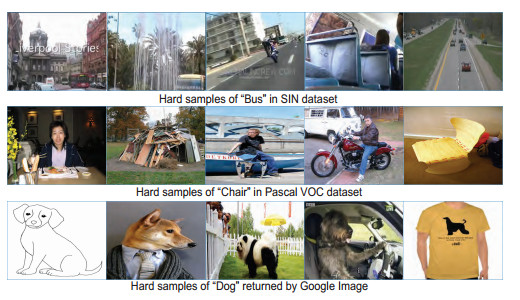
    Citation: Tieliang Gong, Qian Zhao, Deyu Meng, Zongben Xu. Why Curriculum Learning & Self-paced Learning Work in Big/Noisy Data: A Theoretical Perspective[J]. Big Data and Information Analytics, 2016, 1(1): 111-127. doi: 10.3934/bdia.2016.1.111

    Related Papers:

    [1] M Supriya, AJ Deepa . Machine learning approach on healthcare big data: a review. Big Data and Information Analytics, 2020, 5(1): 58-75. doi: 10.3934/bdia.2020005
    [2] Xiangmin Zhang . User perceived learning from interactive searching on big medical literature data. Big Data and Information Analytics, 2017, 2(3): 239-254. doi: 10.3934/bdia.2017019
    [3] Minlong Lin, Ke Tang . Selective further learning of hybrid ensemble for class imbalanced increment learning. Big Data and Information Analytics, 2017, 2(1): 1-21. doi: 10.3934/bdia.2017005
    [4] Nickson Golooba, Woldegebriel Assefa Woldegerima, Huaiping Zhu . Deep neural networks with application in predicting the spread of avian influenza through disease-informed neural networks. Big Data and Information Analytics, 2025, 9(0): 1-28. doi: 10.3934/bdia.2025001
    [5] Yiwen Tao, Zhenqiang Zhang, Bengbeng Wang, Jingli Ren . Motality prediction of ICU rheumatic heart disease with imbalanced data based on machine learning. Big Data and Information Analytics, 2024, 8(0): 43-64. doi: 10.3934/bdia.2024003
    [6] Sunmoo Yoona, Da Kuang, Peter Broadwell, Haeyoung Lee, Michelle Odlum . What can we learn about the Middle East Respiratory Syndrome (MERS) outbreak from tweets?. Big Data and Information Analytics, 2017, 2(3): 203-207. doi: 10.3934/bdia.2017013
    [7] Jason Adams, Yumou Qiu, Luis Posadas, Kent Eskridge, George Graef . Phenotypic trait extraction of soybean plants using deep convolutional neural networks with transfer learning. Big Data and Information Analytics, 2021, 6(0): 26-40. doi: 10.3934/bdia.2021003
    [8] Cai-Tong Yue, Jing Liang, Bo-Fei Lang, Bo-Yang Qu . Two-hidden-layer extreme learning machine based wrist vein recognition system. Big Data and Information Analytics, 2017, 2(1): 59-68. doi: 10.3934/bdia.2017008
    [9] Jian-Bing Zhang, Yi-Xin Sun, De-Chuan Zhan . Multiple-instance learning for text categorization based on semantic representation. Big Data and Information Analytics, 2017, 2(1): 69-75. doi: 10.3934/bdia.2017009
    [10] Jiaqi Ma, Hui Chang, Xiaoqing Zhong, Yueli Chen . Risk stratification of sepsis death based on machine learning algorithm. Big Data and Information Analytics, 2024, 8(0): 26-42. doi: 10.3934/bdia.2024002
  • Since being recently raised, curriculum learning (CL) and selfpaced learning (SPL) have attracted increasing attention due to its multiple successful applications. While currently the rationality of this learning regime is heuristically inspired by the cognitive principle of humans, there still isn't a sound theory to explain the intrinsic mechanism leading to its effectiveness, especially on some successful attempts on big/noise data. To address this issue, this paper presents some theoretical results for revealing the insights under this learning scheme. Specifically, we first formulate a new learning problem aiming to learn a proper classifier from samples generated from the training distribution which is deviated from the target distribution. Furthermore, we find that the CL/SPL regime provides a feasible solving strategy for this learning problem. Especially, by first introducing high-confidence/easy samples and gradually involving low-confidence/complex ones into learning, the CL/SPL process latently minimizes an upper bound of the expected risk under target distribution, purely using the data from the deviated training distribution. We further construct a new SPL learning algorithm based on random sampling, which better complies with our theory, and substantiate its effectiveness by experiments implemented on synthetic and real data.


    1. Introduction

    Recently, curriculum learning (CL) [2] and self-paced learning (SPL) [12] have been attracting increasing attention in machine learning and computer vision. Both learning paradigms are inspired by the learning principle underlying the cognitive process of humans/animals, which generally starts with learning easier aspects of an learning task, and then gradually takes more complex examples into consideration.

    Since being raised, multiple variations of this CL/SPL learning regime, like self-paced reranking [8], self-paced learning with diversity [9], and self-paced curriculum learning [10], have been proposed to further ameliorate its capability. Its effectiveness has also been extensively validated in various machine learning and computer vision tasks, including object detector adaptation [20], dictionary learning [19], long-term tracking [18] and matrix factorization [23]. Especially, this paradigm has been integrated into the system developed by CMU Informedia team, and achieved the leading performance in challenging semantic query (SQ)/000Ex tasks of the TRECVID MED/MER competition organized by NIST in 2014 [22]. Just as indicated by the initial work [2] along this line, two advantages of the CL/SPL learning have been empirically substantiated, especially under big data/noisy scenarios [12,8,9,10,1,11]: generalization improving and convergence speedup.

    Albeit with superior performance in applications, the reasonability of the CL/SPL regime is only intuitively explained by its cognitive understanding, while short of a sound theory to reveal the insightful mechanism leading to its effectiveness. Specifically, current CL/SPL learning methods need to iteratively solve varying optimization problems under gradually increasing pace parameters [12,8,9,10], while there is still not a theoretical argument presented to clarify where these methods converge to and which objective is these methods intrinsically solve.

    To the above issue, this work initializes the learning theory for CL/SPL and provides an insightful explanation for the effectiveness mechanism under this line of learning schemes. Specifically, the main contribution of this paper can be summarized as the following aspects.

    Different from the traditional learning theory assuming the similar training and test distribution, a new theory is formalized to understand the learning problem under the assumption that there exists deviation between training and test/target distributions. This actually is the case often encountered in this era of big data. Nowadays, in various learning tasks like object recognition, event detection and user behavior analysis, learners always need to achieve massive data source for training. In general these massive data are collected and annotated from company users (e.g., the Netflix database1), the web (e.g., the LFW database2) or by making use of crowdsourcing involvement (e.g., the ImageNet database3). The subjective understanding of any annotator is inevitably more-or-less deviated from the objective oracle knowledge underlying data. This naturally conducts the deviation from the training distribution (accumulated from knowledge of all involved annotators) and the true target one, especially in those ambiguous annotated regions. This inspires us to formulate this learning problem and investigate its learning theory.

    1http://www.netflixprize.com/

    2http://www.image-net.org/

    3http://vis-www.cs.umass.edu/lfw/

    Under the premise of the proposed learning theory, the insight of CL/SPL can be rationally explained. Especially, the theory clarifies that the CL/SPL regime actually attempts to minimize an upper bound of the expected risk under target distribution, purely from the data generated from the deviated training distribution. In specific, easy samples in CL/SPL correspond to those in high-confidence annotated area of training distribution, which is also consistent with the high-confidence region of the target distribution (where annotators can easily confirm and agree). Complex ones, however, are more likely to be located in the ambiguous annotated regions, corresponding to the more deviated area between training and target distributions (where users are easily get uncertain or even wrongly cognized). Thus to start training from easy samples by CL/SPL actually simulates learning from the high-confidence target region, while to gradually incrementing complex ones means that the samples residing on ambiguous training regions then come to be involved. Through this process, the faithful information delivered by those high-confidence/easy samples incline to soundly guide the learning towards the expected target, while being less hampered by those low-confidence/complex samples relatively more deviated from the target. This naturally conducts the advantages of SPL, i.e., better generalization to target and faster convergence in a sound manner, as compared to the traditional learning mode, which considers or even emphasizes unreliable low-confidence samples throughout the learning process.

    Besides, based on the proposed theory, we can construct a new CL/SPL learning scheme based on random sampling. This new scheme better complies with the deduced upper bound of the expected risk on the target distribution, and thus can be more faithfully explained by our theory. We also substantiate the effectiveness of the proposed learning scheme by experiments on synthetic dan real data.

    The rest of this paper is organized as follows. Section 2 briefly reviews the related work on CL/SPL. Section 3 introduces the new learning problem and our motivations. Section 4 establishes the main learning theory for this learning problem, and clarifies its intrinsic relationship to CL/SPL. The SPL learning algorithm by random sampling is constructed in Section 5, and evaluated by experiments in Section 6. The paper is then concluded with a future research.


    2. Related work

    Inspired by the learning principle of humans/animals, [2] formulated the curriculum learning paradigm. Its core idea is to iteratively involve samples into learning in sequence, where easy samples are learned first and more complex ones are gradually included when the learner is ready for them. These gradually included sample sequences from easy to complex are called curriculums learned in different grown-up stages of training. In specific, [2] formalized the CL problem as follows. Let Ptrain(z) be the training distribution from which the input data are generated, where z is a random variable representing a sample for the learner (corresponds to a pair of (x,y) for supervised learning). Let 0Wλ(z)1 be the weight superimposed on z at step λ in the curriculum sequence, with the pace parameter 0λ1. The corresponding training distribution at step λ is

    Qλ(z)Wλ(z)Ptrain(z), (1)

    such that ZQλ(z)dz=1, where Z denotes the whole training set. A sequence Qλ(z) can be called a curriculum if it satisfies that both its entropy H(Qλ) and its weight function Wλ(z) are monotonically increasing with respect to the increasing pace λ. This strategy has been empirically evaluated to be helpful in enhancing generalization capability and fastening the convergence speed in multiple applications [17,1].

    To make the CL idea more implementable in applications, [12] first formulated the key principle of CL as a concise optimization model named SPL. The SPL model includes a weighted loss term on all samples and a general SPL regularizer imposed on sample weights. By sequentially optimizing the model with gradually increasing pace parameter on the SPL regularizer, more samples can be automatically included into training from easy to complex in a pure self-paced way. [8] and [23] further built a guideline to construct a rational SPL regularizer, and formalized the SPL model as the following optimization problem:

    minw,v[0,1]nni=1viL(yi,f(xi,w))+r(v;λ), (2)

    where L(y,f(x,w)) denotes the loss between the annotated label y and the estimated one f(x,w), with model parameter w, and vi denotes the binary variable, which indicates whether the i-th sample is easy or not. r(v;λ) is the SPL regularizer. λ is a parameter controlling the learning pace. The larger λ is, the more samples are involved in training and the more "grown-up" the trained model is. Under this guide line, multiple variations of SPL models have been constructed, including self-paced reranking (SPaR) [8], self-paced learning with diversity [9], and self-paced curriculum learning [10], and multiple applications of this SPL framework have been attempted, such as object detector adaptation [20], specific-class segmentation learning [13], visual category discovery [14], long-term tracking [18] and background subtraction [23]. Especially, the SPaR method was integrated into the system developed by CMU Informedia team, and achieved leading performance in challenging SQ/000Ex tasks of the TRECVID MED/MER competition organized by NIST [22].

    In this paper, we attempt to explore the insightful reason behind these successful applications of CL/SPL. To the best of our knowledge, this is the first theoretical explanation work for this newly emerging methodology.


    3. A new understanding for the learning problem in big data sceneries

    The current learning tasks always need to collect a massive data set for training. Such a large magnitude makes it only possible to achieve the expected data from crowdsourcing, especially for supervised learning tasks. This often conducts large amount of ambiguous (or complex in CL/SPL) samples for general users in the obtained data, as illustrated in Figure 1, showing typical "hard" samples from the SIN4 and Pascal VOC5 data sets, and returned by Google image search engine6. The reason is that any participant has his/her own specific viewpoint on a problem as compared to most others, and there is thus inevitably a deviation from each collector/annotator's subjective understanding to the objective oracle knowledge of the problem. This naturally leads to the problem that the training distribution, Ptrain(z), accumulated by all collector/annotator's knowledge, is different from the test/target distribution, Ptarget(z), to which the learning really needs to generalize.

    Figure 1. Some relatively complex samples from the SIN and Pascal VOC data sets, and returned by Google image search engine..

    4http://www.ee.columbia.edu/ln/dvmm/a-TRECVID/

    5http://host.robots.ox.ac.uk/pascal/VOC/

    6https://images.google.com/

    Albeit deviated, useful information under Ptarget(z) can still be explored from Ptrain(z). Most participants share a same common sense on high-confidence samples, and these faithful samples thus tend to be distributed in a region with relatively large density. For supervised learning problem, such region should be located intra-class and relatively far from the classification boundary where samples are easy to be misclassified. In these high-confidence areas, the subjective understanding of humans and the objective knowledge should be consistent and Ptrain(z) and Ptarget(z) should be accordant. Comparatively, those ambiguous/complex samples, conducted by the cognitive differences or even misoperation of annotators, should occupy a relatively smaller proportion in data and located in a region with smaller density. Their locations should be near classification boundary or even inner wrong classes (e.g., noises/outliers) in supervised learning. This naturally leads to an evident heavy-tailed shape of Ptrain(z) as compared to Ptarget(z) in such low-confidence regions, as shown in Figure 2.

    Figure 2. Left: Illustration for the training/target distribution Ptrain(x)/Ptarget(x), as well as a sequence of pace distributions Qλ(x) varying from Ptarget(x) to Ptrain(x). Note that Ptrain(x) has an evident heavy tail as compared to Ptarget(x). Right: The corresponding weight functions with respect to varying pace λ..

    In small/clean sample cases, such a low-confidence region is always with few generated samples due to its small density and small base number of samples. Thus it tends to be configured as a blank "margin" area. Through finding a classification surface to maximize this margin, the decision boundary can always be effectively located [21]. In the premise of practical big/noisy data, however, such margin tends to be very hard to enanchor. Both relatively high density of marginal samples (caused by noise/outliers) and large data cardinality (caused by big data) tend to fill the margin, and the heavy noises/outliers even seriously mislead the margin location. This might explain the fail cases of traditional margin-emphasizing algorithms like SVM [21], Adaboost [7], and etc., in some real data applications [8,9].

    It is thus rational to more emphasize the high-confidence (i.e., easy) samples rather than low-confidence (i.e., complex) ones in certain real data cases, instead of treating the former as non-support-vectors and ignoring their role in learning. This constitutes the basic methodology under CL/SPL, which more complies with the human learning process. Such high-confidence-sample-emphasizing idea has also been employed to build never-ending machine learning systems that acquire the ability to extract structured information from unstructured data [4,15] by persistently picking up high-confidence samples in iteration.

    In sum, our argument is that in real big/noisy data scenarios, both learning theories and implementation methods need to be handled in new viewpoints. In theory, instead of similar [5,6], the target distribution is often deviated from the training, especially in those low-confidence regions; and in implementation, high-confidence samples, i.e., the traditional non-support-vectors, might be put more emphasis in learning, as the CL/SPL methodology suggests.

    In the following, we will provide some preliminary theoretical results on this new setting of learning problem, and deliver a rational theoretical explanation for the working mechanism under CL/SPL methodology.


    4. SPL learning theory


    4.1. Problem setting

    In this work we mainly investigate the binary classification problem. Following the classic setting of learning theory, our aimed learning problem is: Let X be a compact subset of Rd, Y={1,1} be the label set and Z=X×Y be the whole set. The binary classification problem aims at learning a proper classifier f:XY from the input training samples {zi=(xi,yi)}ni=1 generated from the underlying training distribution Ptrain(Z)=Ptrain(X|Y)Ptrain(Y) [6], such that the following expected risk can be minimized:

    R(f):=ZLf(z)Ptarget(x|y)Ptarget(y)dz,

    where Ptarget(Z)=Ptarget(X|Y)Ptarget(Y) denotes the target distribution on Z, and Lf(z)=1f(x)y=1yf(x)2, denoting the loss function measuring the difference between the predicted and true labels. Both Ptrain(Z) and Ptarget(Z) are fixed while unknown. The following empirical risk is thus considered for actual implementation:

    Remp(f)=1nni=1Lf(zi). (3)

    We assume Ptarget(y=1)=Ptrain(y=1)=1/2 for easy evaluation and denote P+train(x)=Ptrain(x|y=1), Ptrain(x)=Ptrain(x|y=1), P+target(x)=Ptarget(x|y=1), Ptarget(x)=Ptarget(x|y=1). Since the deduction for both y=1 and y=1 cases are exactly similar, we only consider one case in the following and denote Ptrain(x) and Ptarget(x) omitting notion +1 or 1.


    4.2. A simulated curriculum format

    We first formulate Ptarget(x) as the weighted expression of Ptrain(x):

    Ptarget(x)=1αWλ(x)Ptrain(x), (4)

    where 0Wλ(x)1 and α=XWλ(x)Ptrain(x)dx denotes the normalization factor7. Based on Eq. (4), Ptarget(x) actually corresponds to a curriculum as defined in Eq. (1) under the weight function Wλ(x). As analyzed in the last section, Wλ(x) should be of small values in the low-confidence area of Ptarget where complex samples are located, while have larger values (close to 1) in the high-confidence area where easy samples reside. This can be easily understood by observing Figure 2.

    7We thus have α1 since Wλ(x)Ptrain(x)Ptrain(x).

    Eq. (4) can be equivalently reformulated as

    Ptrain(x)=αPtarget(x)+(1α)E(x) (5)

    where

    E(x)=11α(1Wλ(x))Ptrain(x).

    Here it is easy to see E(x) is a distribution (XE(x)dx=1) formulated by the weighted Ptrain(x) under the weight function (1Wλ(x)). This term actually measures the deviation from Ptarget to Ptrain. In high-confidence area of Ptarget, E(x) corresponds to the nearly zero-weighted Ptrain, and thus the deviations/errors tend to be small. On the contrary, in the low-confidence area, E(x) imposes relatively large weights on Ptrain, naturally leading to its large deviation values. This complies with our aforementioned analysis on the deviation measure. The more confidently a sample is annotated, the less deviated its label should be from the true one.

    We can then construct the following curriculum sequence for our theoretical evaluation:

    Qλ(x)=αλPtarget(x)+(1αλ)E(x), (6)

    where αλ varies from 1 to α with increasing pace parameter λ. Correspondingly, the curriculum Qλ simulates the changing process from Ptarget to Ptrain, as illustrated in Figure 2. Note that Qλ(x) can also be regularized into the curriculum formulation as Eq. (1) as follows:

    Qλ(x)Wλ(x)Ptrain(x),

    where

    Wλ(x)αλPtarget(x)+(1αλ)E(x)αPtarget(x)+(1α)E(x)

    with 0Wλ(x)1 through normalizing its maximal value as 1.

    Note that the initial stage of this CL process sets WλPtargetPtrain, which is of larger weights in the high-confidence area while much smaller in low-confidence area due to the heavy-tail problem. The weights are thus of more vibrations. With the pace λ increasing, the large weights in high-confidence area become smaller while small ones in low-confidence area become larger, leading to more uniform distributed weights with smaller variations. After normalizing Wλ(x) into the interval [0,1], its values tend to consistently increase in λ, which can be easily understood by Figure 2. This thus complies with the weight-increasing condition defined for a curriculum in [2].

    By taking (6) as the pace distribution, we attempt to present some theoretical results on CL/SPL strategy. These results will help us get some useful insights under this interesting learning scheme.


    4.3. CL/SPL learning theory

    First we need some preliminary definitions.

    Definition 4.1. Let G be a function family mapping from Z to [a,b], P(Z) a distribution on Z and S=(z1,,zm) a set of i.i.d. samples drawn from P. The empirical Rademacher complexity of G with respect to S is then defined by

    ˆRm(G)=Eσ[supgG1mmi=1σig(zi)], (7)

    where σis are i.i.d. samples drawn from the uniform distribution in {1,1}. The Rademacher complexity of G is defined by the expectation of ˆRm(G) over all samples S:

    Rm(G)=ESPm|ˆRS(G)|. (8)

    Definition 4.2. The Kullback-Leibler divergence DKL(pq) between two densities p(Ω) and q(Ω) is defined by

    DKL(pq)=Ωp(x)logp(x)q(x)dx. (9)

    Based on the above definitions, we can estimate the generalization error bound for CL/SPL learning under the curriculum Qλ. Firstly we present the following necessary lemmas for this task.

    Lemma 4.3. (Bretagnolle-Huber inequality) Let p and q be density functions, and then we have

    |p(x)q(x)|dx21exp{DKL(pq)}. (10)

    Lemma 4.4. [16] Let H be a family of function taking value in {1,1} and P be the distribution over the input space X. Then for any δ>0, with confidence at least 1δ over a sample set S, the following holds for any fH:

    R(f)Remp(f)+Rm(H)+ln(1/δ)2m. (11)

    In addition, we have

    R(f)Remp(f)+ˆRm(H)+3ln(2/δ)2m. (12)

    Lemma 4.5. Suppose S{x:xR} be a sample set of size m, and H={xsgn(wTx):minS|wTx|=1wB} be hypothesis class, where wRn, xRn, and then we have

    ˆRm(H)BRm. (13)

    Proof.

    ˆRm(H)=1mEσ[supwBmi=1σisgn(wixi)]1mEσ[supwBmi=1σi|sgn(wixi)|]1mEσ[supwBmi=1σi|wixi|]BmEσ[mi=1σixi]BmEσ[[mi=1σixi2]]12=BmEσ[[mi,j=1σiσj(xixj)2]]12                        Bm[Eσ[mi=1xi2]]12                        =BRm.

    Then we give the main results of this work.

    Theorem 4.6. Suppose {zi}mi=1 are i.i.d. samples drawn from the pace distribution Qλ. Let m+/m be the number of positive/nagetive samples, m=min{m,m+}, and H the function family projecting to {1,1}. Then for any δ>0 and fH, with confidence at least 12δ we have:

    R(f)12R+emp(f)+12Remp(f)+12Rm+(H)+12Rm(H)+ln(1/δ)m+(1αλ)1exp{DKL(P+targetE+)}+(1αλ)1exp{DKL(PtargetE)}, (14)

    and

    R(f)12R+emp(f)+12Remp(f)+12ˆRm+(H)+12ˆRm(H)+3ln(2/δ)m++(1αλ)1exp{DKL(P+targetE+)}+(1αλ)1exp{DKL(PtargetE)}, (15)

    where E+, E denote the error distribution corresponding to P+target, Ptarget, and R+emp(f), Remp(f) denote the empirical risk on positive samples and negative samples, respectively.

    Proof. We first rewrite the expected risk as

    R(f)=ZLf(z)Ptarget(x|y)Ptarget(y)dz=12X+Lf(x,y)Ptarget(x|y=1)dx+12XLf(x,y)Ptarget(x|y=1)dx:=12(R+(f)+R(f)).

    The empirical risk tends not to approximate the expected risk due to the inconsistence of Ptrain and Ptarget. However, by introducing intermediate risk with pace distribution, namely the pace risk, and denoting by EQλ(f) in the error analysis, we can formulate the following error decomposition

    12(R+(f)+R(f))12(R+emp(f)+Remp(f))=12[R+(f)EQ+λ(f)+EQ+λ(f)R+emp(f)]+12[R(f)EQλ(f)+EQλ(f)Remp(f)]:=S1+S2. (16)

    Let S1=A1+A2 and S2=B1+B2, where A1=12(R+(f)EQ+λ(f)), A2=12(EQ+λ(f)R+emp), B1=12(R(f)EQλ(f)), B2=12(EQλ(f)Remp(f)). Here, EQ+λ(f) and EQλ(f) denote the pace risk with respect to positive samples and negative samples, respectively.

    We first focus on the estimation of A1. By the fact the 0-1 loss is bounded by 1, we have

    A112X+(P+target(x)Q+λ(x))dx=12X+(P+target(x)αλP+target(x)(1αλ)E+(x))dx=12(1αλ)X+(P+target(x)E+(x))dx(1αλ)1exp{DKL(P+targetE+)} (17)

    The last inequality is obtained by Lemma 4.3. For the estimation of A2, according to Lemma 4.4, the following holds with confidence 1δ

    A212Rm+(H)+12ln(1/δ)2m+. (18)

    In the similar way, we can bound B1 and B2 as follows

    B1(1αλ)1exp{DKL(PtargetE)}, (19)

    and

    B212Rm(H)+12ln(1/δ)2m. (20)

    By taking m=min{m+,m} and combining Eqs. (17) (18) (19) (20), we can easily get Eq. (14). In addition, one can further get:

    Rm(H)ˆRm(H)+ln(2/δ)2m. (21)

    By replacing Rm(H) in Eq. (14) with Eq. (21), we have (15).

    The proof is then completed.

    Note that the above established error bounds upon 0-1 loss are hard to optimize. We thus further deduce another bound under the commonly utilized hinge loss.

    Corollary 1. Suppose {(xi,yi)}mi=1(X×{1,1}) are i.i.d. samples drawn from the pace distribution Qλ with radius |X|R. Denote m+/m be the number of positive/nagetive samples and m=min{m,m+}. Let H={xwTx:minS|wTx|=1wB}, and ϕ(t)=(1t)+ for tR be the hinge loss function. Then for any δ>0 and gH, with confidence at least 12δ, it holds that:

    R(sgn(g))12m+m+i=1ϕ(yig(xi))+12mmi=1ϕ(yig(xi))+RBm+3ln(1/δ)m+(1αλ)1exp{DKL(P+targetE+)}+(1αλ)1exp{DKL(PtargetE)}. (22)

    Proof. Based on Lemma 4.5 to Eq. (15), and the fact that the hinge loss is the upper bound of 01 loss, we can then obtain the result.

    Note that there are three components in the upper bound of the expected risk under Ptarget. The first row corresponds to the empirical risk on training samples generated from Qλ. With λ increasing, these samples start by mainly generating from high-confident (easy) area of Ptarget in probability and gradually involve more complex ones. The second row reflects the approximation capability of training samples to evaluate information of Qλ. The more samples are considered, the smaller this term is and the better approximation can be achieved. The last two rows measure the generalization capability of the learned classifier, which is monotonically increasing with respect to both the KL-divergence between the error distribution E and the target Ptarget, and the pace parameter λ. That is, the more deviated is the error E from Ptarget, the more difficult is to learn a proper classifier from training data which can generalize well on Ptarget. Also, in the late stage of CL/SPL (corresponding to large λ), the generalization of the learned classifier tends to be worse due to the gradually more evident deviation from the curriculum Qλ to Ptarget. The last two terms actually compromise the approximation and generalization capabilities of this CL/SPL process with Qλ.

    This theory reveals the following insights underlying this CL/SPL process. The "easy-to-complex" property of the curriculum Qλ intrinsically facilitates the information transfer from Ptrain to Ptarget, and makes it feasible to approximate the solution of the learning problem as set in Section 4.1, i.e., to learn a classifier with minimal expected risk on Ptarget through the empirical risk on training samples generated from Ptrain. In specific, we can approach the task of minimizing the expected risk on Ptarget by gradually increasing the pace λ, generating relatively high-confidence (easy) samples from Qλ, and minimizing the empirical risk on these samples. This complies with the core idea under previous CL/SPL regimes. It is interesting that the previous investigations attribute the advantage of CL/SPL by that its performance is soundly guided by the faithful easy samples, while our theory further reveals that this regime facilitates learning to approach a good generalization to the target distribution.


    5. SPL insight: Approximate rational curriculums from training data


    5.1. Simulate Qλ from training samples

    When we only have samples {(xi,yi)}ni=1X×{1,1} generated from Ptrain, we can approximately simulate a rational Qλ as Eq. (6) in the following way. For easy discussion, we still only consider either of +1 and 1 cases, and ignore the notion +1 or 1.

    First, let's approximate ˆPtrain=piδxi(x), where δxi(x) denotes the Dirac delta function centered at xi and pi=1m. It is easy to see that ˆPtrain supposes a uniform density on each sample xi. Next, in the beginning λ paces, we impose a smaller weights vi(λ) on low-confidence samples located near inter-class boundary than those on high-confidence regions to formulate the initial ˆQλ(x)ni=1vi(λ)piδxi(x). By dominantly suppressing the heavy-tailed region of ˆPtrain, i.e., by putting nearly zero weights vi(λ) on those evident low-confidence samples, ˆQ0 is expected to form a rational approximation to Ptarget. We then increase the pace λ to gradually increase the small weight vi(λ) to 1. The corresponding ˆQλ(x)ni=1vi(λ)piδxi(x) then approximates a curriculum sequence varying from ˆQ0 to ˆPtrain like Eq. (6).


    5.2. Revisit previous SPL models

    Instead of minimizing the empirical risk Remp(f) as illuminated in our theory, let's minimize its expected value under ˆQλ as:

    minwEˆQλ(1nni=1L(yi,f(xi,w)))=EˆQλL(y,f(x,w))minwivi(λ)L(yi,f(xi,w)), (23)

    where the first expectation is taken with respect to {xi}ni=1 which are i.i.d samples drawn from ˆQλ. As analyzed above, vi(λ) should satisfy: (1) Under fixed λ, vi(λ) is monotonically increasing with its confidence degree; (2) For each sample xi, vi(λ) is monotonically increasing with respect to the pace λ.

    An useful knowledge to judge whether the label confidence of a sample is high or low is through its learning error. That is, the high-confidence sample tends to be located inside the region of its category, thus always leading to its small training error, and vice versa. From this understanding, Eq. (23) exactly corresponds to current SPL learning models [8,23,10], which fit these weight values to accord with the similar requirements through supplementing a self-paced regularizer on vi(λ) in Eq. (23), as shown in the previous SPL model (2).

    In this sense, we might explain the effectiveness of the previous SPL models by the following insight. Based on our theoretical results, this learning scheme tends to learn from the deviated training information to discover ground truth knowledge of the target distribution, through learning in a sound manner from high-confidence/easy/small-loss samples to low-confidence/complex/large-loss ones. Throughout this learning process, it intrinsically tries to minimize an upper bound of the expected risk on the target distribution, through being terminated at a proper compromised pace. This fully complies with the experience of its real implementations in multiple applications [8,9,23].


    5.3. SPL with random sampling

    Note that current SPL models are all deterministic, while the empirical risk in the upper bound (22) is calculated on randomly generated samples. We thus want to build a new SPL algorithm by using random sampling mechanism. The core idea is to approximate the pace distribution Qλ by imposing weights on samples, and then sampling from this distribution to form new SPL training samples.

    The implementation details are as follows. At each iteration, we first compute the losses of all training samples based on the current model. Then we solve the following optimization problem to form weights on all samples:

    minvni=1viL(yi,f(xi,w))+r(v,λ), (24)

    where r(v,λ) is the self-paced regularizer as defined in Eq. (2). After that, we normalize v by v/v1 to construct the empirical pace distribution ˆQλ(x)=vi(λ)piδxi(x), and then redraw samples from the training set according to ˆQλ. A new model is then recursively trained on these samples. The whole process is summarized in Algorithm 1.

    Table . .
    Algorithm 1 Self-Pace Learning with Random Sampling (RS-SPL)
    Input: training data D={xi,yi}ni=1, initial pace parameter λ,m and stepsize μ,k.
    Output: model parameter w.
    1:Train a model on entire training set to obtain loss {L(yi,f(xi,w))}ni=1.
    2:repeat
    3:Solve (24) to obtain v(λ).
    4:v(λ)=v(λ)/v(λ)1.
    5:Draw m samples from ni=1vi(λ)piδxi(x) to form Dλ.
    6:Train a new model on Dλ to obtain w.
    7:If λ is small, increase λ by μ and increase m by k.
    8:until stopping criteria satisfied
     | Show Table
    DownLoad: CSV

    There are many choices for r(v,λ) based on three axiomic conditions defined on it [8]. We just readily use the following due to its easiness and effectiveness:

    r(v,λ)=γni=1log(vi+1λγ), (25)

    where γ>0 is a tuning parameter. The optimal v(λ) to (24) can be analytically computed by

    vi(λ)={1logγlog(L(yi,f(xi,w))+γ)L(yi,f(xi,w))<λ0L(yi,f(xi,w))λ.

    6. Experiments

    In this section, we implemented experiments on synthetic and real classification datasets. The linear SVM, implemented by LibSVM [3], is utilized as the comparison method.


    6.1. A synthetic example

    We first give a synthetic example to illustrate behavior of the proposed RS-SPL algorithm. The data were generated as follows: Two 2-D Gaussian distributions, each associated with a class, were specified as the target distribution. The training distribution is further mixed with another two 2-D Gaussian distributions, each centered at the low density area of the target distribution of corresponding class to enforce deviation. We generated 2000 clean training samples, 1000 per class, and 2000 test samples from the target distributions. Then 400 samples from the deviated distributions, 200 per class, were added to the training set. The resulted training and test samples are shown in Figure 3.

    Figure 3. Samples used in our synthetic experiment. Left: Training samples. Triangles and squares are sampled from the target distribution, and crosses and pluses from the deviated distribution. Right: Test samples, generated from the target distribution..

    In order to understand the behavior of RS-SPL, we implemented Algorithm 1 to this synthetic data and plot in Figure 4 the selected samples and the learned separating hyperplane during the SPL process. It can be observed that, samples from the high density region of the training distribution are selected first. As the SPL iteration continues, more and more samples with comparatively high confidence are included for training the classifier, and the separating hyperplane tends to be learned more accurately. However, when "hard" samples, i.e., those deviated samples, are included at the latter stages of SPL, the learned hyperplane tends to be disordered. Such behavior can also be substantiated by the accuracy tendency on the test data as shown in Figure 5. These results coincide with the SPL learning theory developed in Section 4, which asserts that the optimal expected risk tends to be achieved as a tradeoff between the better approximation capability of increasingly more samples and the worse generalization derived by the divergence from the pace distribution to the target.

    Figure 4. Upper: The selected training samples and the learned separating hyperplane (black line) in SPL iterations. Lower: Corresponding performance on the test samples..
    Figure 5. Classification accuracy (%) with respect to the SPL iteration in synthetic experiment..

    6.2. Real data evaluation

    We also implemented the proposed method to 5 real-world classification datasets, including magic8, image, waveform, ringnorm and twonorm9. The numbers of instances and features of each dataset are summarized in Table 1.

    Table 1. Statistics of 5 utilized real classification datasets..
    Dataset # Instances # Features
    magic 19020 10
    waveform 5000 21
    image 2310 18
    ringnorm 7400 20
    twonorm 7400 20
     | Show Table
    DownLoad: CSV

    8http://archive.ics.uci.edu/ml/datasets.html

    9http://www.raetschlab.org/Members/raetsch/benchmark

    We randomly split each dataset into two subsets with equal sizes for training and testing, respectively. Then we applied the proposed RS-SPL algorithm to training a SVM classifier on the training set, and evaluated its performance in terms of classification accuracy on the test set. The parameters for SVM and RS-SPL were selected via hold-out validation on training set. We averaged the performance for each dataset over 50 runs as summarized in Table 2. As a comparison, we also include the results of the batch-trained SVM. We can see that the proposed SP-SPL algorithm can improve the classification accuracy over batch training. Its effectiveness can thus be validated.

    Table 2. Classification accuracy (%) on 5 real-world classification datasets. The results are averaged over 50 runs..
    Dataset # Batch Train # SPL Train
    magic 79.13±0.28 79.74±0.77
    waveform 88.05±0.52 88.30±0.53
    image 84.46±1.11 86.26±1.07
    ringnorm 77.09±0.63 77.36±0.59
    twonorm 97.71±0.20 97.81±0.17
     | Show Table
    DownLoad: CSV

    7. Conclusion

    We have presented a theoretical explanation for the working insight underlying the CL/SPL paradigm. Specifically, we clarify that the insight of the CL/SPL strategy is to learn knowledge of the target information from the given samples generated from the training distribution, which is deviated from the target. We have also argued that such a learning problem tends to happen in real big data scenarios due to the bias between subjective understanding of data collectors/annotators and objective oracle knowledge underlying data. Besides, our theory suggests the importance of high-confidence/easy samples in learning, which are generally taken as non-support-vectors in traditional learning methods and whose role is more or less underestimated. We further designed a new SPL algorithm with random sampling, which better complies our theory, and verified its effectiveness by experiments on synthetic and real data.

    Our future research includes designing feasible termination condition for CL/SPL iteration based on our theory, deriving theory under unequal probabilities between P(y=1) and P(y=1), making the upper bound tighter, and applying the RS-SPL algorithm to more realistic big data sets.


    [1] [ S. Basu and J. Christensen, Teaching Classification Boundaries to Humans, Proceddings of the 27th AAAI Conference on Artificial Intelligence, 2013.
    [2] [ Y. Bengio, J. Louradour, R. Collobert and J. Westone, Curriculum Learning, Proceedings of the 26th International Conference on Machine Learning, (2009), 41-48.
    [3] [ C.-C. Chang and C.-J. Lin, LIBSVM:A library for support vector machines, ACM Transactions on Intelligent Systems and Technology, 2(2011), 1-27. Software available from:http://www.csie.ntu.edu.tw/~cjlin/libsvm.
    [4] [ X. Chen, A. Shrivastava and A. Gupta, NEIL:Extracting visual knowledge from web data, Proceedings of the IEEE International Conference on Computer Vision, (2013), 1409-1416.
    [5] [ F. Cucker and S. Smale, On the mathematical foundations of learning, Bull. Amer. Math. Soc., 39(2002), 1-49.
    [6] [ F. Cucker and D. X. Zhou, Learning Theory:An Approximation Theory Viewpoint, Cambridge University Press, New York, NY, USA, 2007.
    [7] [ Y. Freund and R. E. Schapire, Experiments with a new boosting algorithm, Proceedings of the 13th International Conference on Machine Learning, 1996.
    [8] [ L. Jiang, D. Y. Meng, T. Mitamura and A. Hauptman, Easy samples first:Self-paced reranking for multimedia search, Proceddings of the ACM International Conference on Multimedia, (2014), 547-556.
    [9] [ L. Jiang, D. Y. Meng, S. Yu, Z. Z. Lan, S. G. Shan and A. Hauptma, Self-paced Learning with Diversity, Advances in Nerual Information Processing Systems 27, 2014.
    [10] [ L. Jiang and D. Y. Meng, Q. Zhao, S. G. Shan and A. Hauptman, Self-paced Curriculum Learning, Proceddings of the 29th AAAI Conference on Artificial Intelligence, 2015.
    [11] [ F. Khan, X. Zhu and B. Mutlu, How do Humans Teach:On Curriculum Learning and Teaching Dimension, Advances in Nerual Information Processing Systems 24, 2011.
    [12] [ M. Kumar, B. Packer and D. Koller, Self-paced Learning for Latent Variable Models, Advances in Nerual Information Processing Systems 23, 2010.
    [13] [ M. Kumar, H. Turki, D. Preston and D. Koller, Learning specfic-class segmentation from diverse data, Proceedings of the IEEE International Conference on Computer Vision, 2011.
    [14] [ Y. Lee and K. Grauman, Learning the easy things first:Self-paced visual category discovery, Proceedings of the IEEE Conference on Computer Vision and Pattern Recognition, (2011), 1721-1728.
    [15] [ T. Mitchell, W. Cohen, E. Hruschka, P. Talukdar, J. Betteridge, A. Carlson, B. Dalvi, M. Gardner, B. Kisiel, J. Krishnamurthy, N. Lao, K. Mazaitis, T. Mohamed, N. Nakashole, E. Platanios, A. Ritter, M. Samadi, B. Settles, R. Wang, D. Wijaya, A. Gupta, X. Chen, A. Saparov, M. Greaves and J. Welling, Never-Ending Learning, Proceddings of the 29th AAAI Conference on Artificial Intelligence, 2015.
    [16] [ M. Mohri, A. Rostamizadeh and A. Talwalkar, Foundations of Machine Learning, The MIT Press, Cambridge, Massachusetts, London, England, 2012.
    [17] [ E. Ni and C Ling, Supervised learning with minimal effort, Advances in Knowledge Discovery and Data Mining, 6119(2010), 476-487.
    [18] [ J. Supanvcivc and D. Ramana, Self-paced learning for long-term tracking, Proceedings of the IEEE Conference on Computer Vision and Pattern Recognition, 2013.
    [19] [ Y. Tang, Y. B. Yang and Y. Gao, Self-paced Dictionary Learning for Image Classification, Proceddings of the ACM International Conference on Multimedia, (2012), 833-836.
    [20] [ K. Tang, V. Ramanathan, F. Li and D. Koller, Shifting weights:Adapting object detectors from image to video, Advances in Nerual Information Processing Systems 25, 2012.
    [21] [ V. Vapnik, Statistical Learning Theory, Wiley-Interscience, New York, 1998.
    [22] [ S. Yu, L. Jiang, Z. Mao, X. J. Chang, X. Z. Du, C. Gan, Z. Z. Lan, Z. W. Xu, X. C. Li, Y. Cai, A. Kumar, Y. Miao, L. Martin, N. Wolfe, S. C. Xu, H. Li, M. Lin, Z. G. Ma, Y. Yang, D. Y. Meng, S. G. Shan, P. D. Sahin, S. Burger, F. Metze, R. Singh, B. Raj, T. Mitamura, R. Stern and A. Hauptmann, CMU-Informedia@TRECVID 2014 Multimedia Event Detection (MED), TRECVID Video Retrieval Evaluation Workshop, 2014.
    [23] [ Q. Zhao, D. Y. Meng, L. Jiang, Q. Xie, Z. B. Xu and A. Hauptman, Self-paced Matrix Factorization, Proceddings of the 29th AAAI Conference on Artificial Intelligence, 2015.
  • This article has been cited by:

    1. Manuel Garcia-Piqueras, José Hernández-Orallo, 2021, Chapter 43, 978-3-030-86485-9, 705, 10.1007/978-3-030-86486-6_43
    2. Xin Wang, Yudong Chen, Wenwu Zhu, A Survey on Curriculum Learning, 2021, 0162-8828, 1, 10.1109/TPAMI.2021.3069908
    3. Mobarakol Islam, Lalithkumar Seenivasan, S. P. Sharan, V. K. Viekash, Bhavesh Gupta, Ben Glocker, Hongliang Ren, Paced-curriculum distillation with prediction and label uncertainty for image segmentation, 2023, 1861-6429, 10.1007/s11548-023-02847-9
    4. Melike Nur Yeğin, Ömer Kurttekin, Serkan Kaan Bahşi, Mehmet Fatih Amasyali, Training with growing sets: A comparative study, 2022, 39, 0266-4720, 10.1111/exsy.12961
    5. Yuwei Zhou, Hong Chen, Zirui Pan, Chuanhao Yan, Fanqi Lin, Xin Wang, Wenwu Zhu, 2022, CurML: A Curriculum Machine Learning Library, 9781450392037, 7359, 10.1145/3503161.3548549
    6. Chenkang Zhang, Wanli Shi, Lei Luo, Bin Gu, 2023, Doubly Robust AUC Optimization against Noisy and Adversarial Samples, 9798400701030, 3195, 10.1145/3580305.3599316
    7. Zean Liu, Yuanzhi Cheng, Shinichi Tamura, Multi-Label Local to Global Learning: A Novel Learning Paradigm for Chest X-Ray Abnormality Classification, 2023, 27, 2168-2194, 4409, 10.1109/JBHI.2023.3281466
    8. Kaiyue Liu, Yun Zhou, Hongbin Huang, Bayesian network structure learning with a new ensemble weights and edge constraints setting mechanism, 2024, 2199-4536, 10.1007/s40747-024-01485-1
    9. Peng Zheng, Yong Dou, Yeqing Yan, Sensing the diversity of rumors: Rumor detection with hierarchical prototype contrastive learning, 2024, 61, 03064573, 103832, 10.1016/j.ipm.2024.103832
    10. Zihao Suo, Shanliang Pan, 2025, Chapter 11, 978-981-96-2070-8, 141, 10.1007/978-981-96-2071-5_11
  • Reader Comments
  • © 2016 the Author(s), licensee AIMS Press. This is an open access article distributed under the terms of the Creative Commons Attribution License (http://creativecommons.org/licenses/by/4.0)
通讯作者: 陈斌, bchen63@163.com
  • 1. 

    沈阳化工大学材料科学与工程学院 沈阳 110142

  1. 本站搜索
  2. 百度学术搜索
  3. 万方数据库搜索
  4. CNKI搜索

Metrics

Article views(4319) PDF downloads(584) Cited by(10)

Article outline

Other Articles By Authors

/

DownLoad:  Full-Size Img  PowerPoint
Return
Return

Catalog