Analysis of the current status of TB transmission in China based on an age heterogeneity model

Chuanqing Xu; Kedeng Cheng; Yu Wang; Maoxing Liu; Xiaojing Wang; Zhen Yang; Songbai Guo; Chuanqing Xu; Kedeng Cheng; Yu Wang; Maoxing Liu; Xiaojing Wang; Zhen Yang; Songbai Guo

doi:10.3934/mbe.2023850

Mathematical Biosciences and Engineering

2023, Volume 20, Issue 11: 19232-19253. doi: 10.3934/mbe.2023850

Previous Article Next Article

Research article Special Issues

Analysis of the current status of TB transmission in China based on an age heterogeneity model

1.
School of Science, Beijing University of Civil Engineering and Architecture, 100044, China
2.
Beijing Changping District TB Control Center, 102202, China

Received: 06 July 2023 Revised: 16 September 2023 Accepted: 20 September 2023 Published: 16 October 2023

Tuberculosis (TB) is an infectious disease transmitted through the respiratory system. China is one of the countries with a high burden of TB. Since 2004, an average of more than 800,000 cases of active TB has been reported each year in China. Analyzing the case data from 2004 to 2018, we found significant differences in TB incidence by age group. A model of TB is put forward to explore the effect of age heterogeneity on TB transmission. The nonlinear least squares method is used to obtain the key parameters in the model, and the basic reproduction number R_v = 0.8017 is calculated and the sensitivity analysis of R_v to the parameters is given. The simulation results show that reducing the number of new infections in the elderly population and increasing the recovery rate of elderly patients with the disease could significantly reduce the transmission of TB. Furthermore, the feasibility of achieving the goals of the World Health Organization (WHO) End TB Strategy in China is assessed, and we obtained that with existing TB control measures it will take another 30 years for China to reach the WHO goal to reduce 90% of the number of new cases by the year 2049. However, in theory it is feasible to reach the WHO strategic goal of ending TB by 2035 if the group contact rate in the elderly population can be reduced, though it is difficult to reduce the contact rate.
- tuberculosis (TB),
- age heterogeneity,
- basic reproduction number,
- sensitivity analysis,
- partial rank correlation coefficient analysis
Citation: Chuanqing Xu, Kedeng Cheng, Yu Wang, Maoxing Liu, Xiaojing Wang, Zhen Yang, Songbai Guo. Analysis of the current status of TB transmission in China based on an age heterogeneity model[J]. Mathematical Biosciences and Engineering, 2023, 20(11): 19232-19253. doi: 10.3934/mbe.2023850

Related Papers:

Abstract

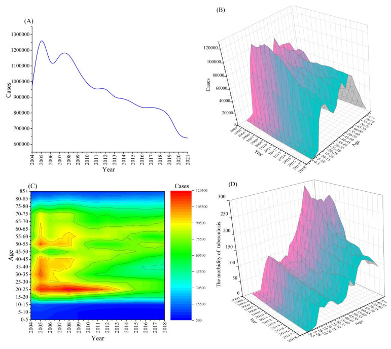
Tuberculosis (TB) is an infectious disease transmitted through the respiratory system. China is one of the countries with a high burden of TB. Since 2004, an average of more than 800,000 cases of active TB has been reported each year in China. Analyzing the case data from 2004 to 2018, we found significant differences in TB incidence by age group. A model of TB is put forward to explore the effect of age heterogeneity on TB transmission. The nonlinear least squares method is used to obtain the key parameters in the model, and the basic reproduction number R_v = 0.8017 is calculated and the sensitivity analysis of R_v to the parameters is given. The simulation results show that reducing the number of new infections in the elderly population and increasing the recovery rate of elderly patients with the disease could significantly reduce the transmission of TB. Furthermore, the feasibility of achieving the goals of the World Health Organization (WHO) End TB Strategy in China is assessed, and we obtained that with existing TB control measures it will take another 30 years for China to reach the WHO goal to reduce 90% of the number of new cases by the year 2049. However, in theory it is feasible to reach the WHO strategic goal of ending TB by 2035 if the group contact rate in the elderly population can be reduced, though it is difficult to reduce the contact rate.

References

[1]	Public Health Sciences Data Center. Available from: http://www.phsciencedata.cn.
[2]	H. M. Zhao, Health education in the prevention and treatment of TB, World Latest Med. Inf., 18 (2018), 197–199. https://doi.org/10.19613/j.cnki.1671-3141.2018.51.110 doi: 10.19613/j.cnki.1671-3141.2018.51.110
[3]	Chinese Center for Disease Control and Prevention. Available from: http://www.chinatb.org.
[4]	World Health Organization, Global TB Report (2013). Available from: http://www.who.int/tb/publications/globalreport/en/.
[5]	R. M. G. J. Houben, N. A. Menzies, T. Sumner, G. H. Huynh, N. Arinaminpathy, J. D. Goldhaber-Fiebert, et al., Feasibility of achieving the 2025 WHO global TB target in South Africa, China, and India: a combined analysis of 11 mathematical models, Lancet Global Health, 4 (2016), e806–e815. https://doi.org/10.1016/S2214-109X(16)30199-1 doi: 10.1016/S2214-109X(16)30199-1
[6]	H. Waaler, A. Geser, S. Andersen. The use of mathematical models in the study of the epidemiology of TB, Am. J. Public Health, 52 (1962), 1002–1013. https://doi.org/10.2105/ajph.52.6.1002 doi: 10.2105/AJPH.52.6.1002
[7]	S. Brogger, Systems analysis in TB control: a model, Am. Rev. Respir. Dis., 95 (1967), 419–434. https://doi.org/10.1164/arrd.1967.95.3.419 doi: 10.1164/arrd.1967.95.3.419
[8]	C. S. Revelle, W. R. Lynn, F. Feldmann, Mathematical models for the economic allocation of TB control activities in developing nations, Am. Rev. Respir. Dis., 96 (1967), 893–909. https://doi.org/10.1164/arrd.1967.96.5.893 doi: 10.1164/arrd.1967.96.5.893
[9]	V. Moreno, B. Espinoza, K. Barley, M. Paredes, D. Bichara, A. Mubayi, et al., The role of mobility and health disparities on the transmission dynamics of TB, Theor. Biol. Med. Modell., 14 (2017). https://doi.org/10.1186/s12976-017-0049-6 doi: 10.1186/s12976-017-0049-6
[10]	A. Koch, H. Cox, V. Mizrahi, Drug-resistant TB: challenges and opportunities for diagnosis and treatment, Curr. Opin. Pharmacol., 42 (2018), 7–15. https://doi.org/10.1016/j.coph.2018.05.013 doi: 10.1016/j.coph.2018.05.013
[11]	Y. J. Lin, C. M. Liao, Seasonal dynamics of TB epidemics and implications for multidrug-resistant infection risk assessment, Epidemiol. Infect., 142 (2014), 358–370. https://doi.org/10.1017/S0950268813001040 doi: 10.1017/S0950268813001040
[12]	H. X. Wang, L. Q. Jiang, G. H. Wang, Stability of a TB model with a time delay in transmission, J. North Univ. China, 35 (2014), 238–242. https://doi.org/10.3969/j.issn.1673-3193.2014.03.003 doi: 10.3969/j.issn.1673-3193.2014.03.003
[13]	T. Cohen, M. Lipsitch, R. P. Walensky, M. Murray, Beneficial and perverse effects of isoniazid preventive therapy for latent TB infection in HIV-TB co-infected populations, PNAS, 103 (2006), 7042–7047. https://doi.org/10.1073/pnas.0600349103 doi: 10.1073/pnas.0600349103
[14]	Y. Wang, The fifth national TB epidemiological survey in 2010, Chin. J. Antituberc., 8 (2012), 485–508.
[15]	J. P. Smith, S. Strauss, Y. H. Zhao, Healthy aging in China, J. Econ. Ageing, 4 (2014), 37–43. https://doi.org/10.1016/j.jeoa.2014.08.006 doi: 10.1016/j.jeoa.2014.08.006
[16]	J. A. Jacquez, C. P. Simon, J. Koopman, L. Sattenspiel, T. Perry, Modeling and analyzing HIV transmission: the effect of contact patterns, Math. Biosci., 92 (1988), 119–199. https://doi.org/10.1016/0025-5564(88)90031-4 doi: 10.1016/0025-5564(88)90031-4
[17]	J. P. Millet, E. Shaw, À. Orcau, M. Casals, J. M. Miró, J. A. Caylà, et al., TB recurrence after completion treatment in a European city: reinfection or relapse, PLoS One, 8 (2013), e64898. https://doi.org/10.1371/journal.pone.0064898 doi: 10.1371/journal.pone.0064898
[18]	China Population Statistic Yearbook (2021). Available from: http://www.stats.gov.cn/tjsj/ndsj/.
[19]	Y. Zhao, M. Li, S. Yuan, Analysis of transmission and control of TB in mainland China, 2005–2016, based on the age-structure mathematical model, Int. J. Environ. Res. Public Health, 14 (2017), 1192. https://doi.org/10.3390/ijerph14101192 doi: 10.3390/ijerph14101192
[20]	J. Wang, Can BCG vaccine protect you for life, Fam. Med., 3 (2015), 14.
[21]	National Scientific Data Sharing Platform for Population and Health (2021). Available from: https://www.ncmi.cn.
[22]	S. M. Blower, A. R. Mclean, T. C. Porco, P. M. Small, P. C. Hopewell, M. A. Sanchez, et al., The intrinsic transmission dynamics of TB epidemics, Nat. Med., 1 (1995) 815–821. https://doi.org/10.1038/nm0895-815 doi: 10.1038/nm0895-815
[23]	J. M. Read, J. Lessler, S. Riley, S. Wang, L. J. Tan, K. O. Kwok, et al., Social mixing patterns in rural and urban areas of southern China, Proc. Biol. Sci., 1785 (2014), 281. https://doi.org/10.1098/rspb.2014.0268 doi: 10.1098/rspb.2014.0268
[24]	S. Cheng, E. Liu, F. Wang, Y. Ma, L. Zhou, L. Wang, et al., Systematic review and implemention progress of DOTS strategy, Chin. J. Antituberc., 34 (2012), 585–591.
[25]	Z. L. Feng, J. W. Glasser, A. N. Hill, M. A. Franko, R. Carlsson, H. Hallander, et al., Modeling rates of infection with transient maternal antibodies and waning active immunity: application to Bordetella pertussis in Sweden, J. Theor. Biol., 356 (2014), 123–132. https://doi.org/10.1016/j.jtbi.2014.04.020 doi: 10.1016/j.jtbi.2014.04.020
[26]	C. Fraser, C. A. Donnelly, S. Cauchemez, W. P. Hanage, M. D. Van Kerkhove, T. Déirdre Hollingsworth, et al., Pandemic potential of a strain of Influenza A (H1N1): early findings, Science, 324 (2009), 1557–1561. https://doi.org/10.1126/science.1176062 doi: 10.1126/science.1176062
[27]	P. V. D Driessche, J. Watmough, Reproduction numbers and sub-threshold endemic equilibria for compartmental models of disease transmission, Math. Biosci., 180 (2002), 29–48. https://doi.org/10.1016/s0025-5564(02)00108-6 doi: 10.1016/S0025-5564(02)00108-6
[28]	D. Gao, Y. Lou, D. He, T. C. Porco, Y. Kuang, G. Chowell, et al., Prevention and control of Zika as a mosquito-borne and sexually transmitted disease: a mathematical modeling analysis, Sci. Rep., 6 (2016), 28070. https://doi.org/10.1038/srep28070 doi: 10.1038/srep28070
[29]	L. K. Yan, Application of correlation coefficient and biased correlation coefficient in related analysis, J. Yunnan Univ. Finance Econ., 3 (2003), 78–80. https://doi.org/10.16537/j.cnki.jynufe.2003.03.018 doi: 10.16537/j.cnki.jynufe.2003.03.018
[30]	World Health Organization, WHO End TB Strategy (2014). Available from: https://www.who.int/teams/global-tuberculosis-programme/the-end-tb-strategy.
[31]	G. H. Huynh, D. J. Klein, D. P. Chin, B. G. Wagner, P. A. Eckhoff, R. Liu, et al. TB control strategies to reach the 2035 global targets in China: the role of changing demographics and reactivation disease, BMC Med., 13 (2015), 88. https://doi.org/10.1186/s12916-015-0341-4 doi: 10.1186/s12916-015-0341-4
[32]	E. Ziv, C. L. Daley, S. M. Blower, Early therapy for latent TB infection, Am. J. Epidemiol., 153 (2001), 381–385. https://doi.org/10.1093/aje/153.4.381 doi: 10.1093/aje/153.4.381
[33]	E. Ziv, C. L. Daley, S. M. Blower, Potential public health impact of new TB vaccines, Emerging Infect. Dis., 10 (2004), 1529–1535. https://doi.org/10.3201/eid1009.030921 doi: 10.3201/eid1009.030921
[34]	A. Z. Guo, Control and decontamination of TB in animals, in 2019 International Symposium on Human-Veterinary Diseases and China Rabies Annual Meeting, Hefei, China,
[35]	X. Y. Zhang, M. J. Sun, W. X. Fan, The spread and control of bovine TB, China Anim. Health Inspection, 34 (2017), 70–74.
[36]	Y. Y. Chen, H. C. Chen, A. Z. Guo, Epidemiological characteristics of bovine TB and its prevention and control, China Animal Health, 14 (2012), 7–9.
[37]	L. J. Liu, X. Q. Zhao, Y. C. Zhou, A TB model with seasonality, Bull. Math. Biol., 72 (2010), 931–952. https://doi.org/10.1007/s11538-009-9477-8 doi: 10.1007/s11538-009-9477-8
[38]	O. Diekmann, J. A. Heesterbeek, J. A. Metz, On the definition and the computation of the basic reproduction ratio R0 in models for infectious diseases in heterogeneous populations, J. Math. Biol., 28 (1990), 365–382. https://doi.org/10.1007/BF00178324 doi: 10.1007/BF00178324

Reader Comments

Your name:*

Email:*
© 2023 the Author(s), licensee AIMS Press. This is an open access article distributed under the terms of the Creative Commons Attribution License (http://creativecommons.org/licenses/by/4.0)