Socio-economic determinants of landslide risk perception in Murree hills of Pakistan

$\beta$: Target reliability; $X$: Random variable; ${\mu }_{X}$: The mean of$X$; $d$: Deterministic design variable; GMSE: Generalized mean square cross-validation error; SORA: Sequential optimization and reliability assessment; SVM: Support vector machine; DDV: Deterministic design variable; SVR: Support vector regression; MCC: Multiple correlation coefficient; RBDO: Reliability-based design optimization; MCS: Monte Carlo simulation; DRM: Dimensionality reduction methods; RBF: Radial basis functions; RAAE: Relative average absolute error; LHD: Latin hypercube design; RMSE: Root mean squared error; FFD: Full factorial design; RRMSE: Relative root mean squared error; KKT: Karush Kuhn Tucker; RMAE: Relative maximum absolute error; VF: Variable fidelityFORM: First-order reliability methods; LF: Low fidelity; CBS: Constraint boundary sampling; HF: High fidelity; EGRA: Efficient global reliability analysis; LAS: Local adaptive sampling; EGO: Efficient global optimization; MPP: Most possible point; PRS: Polynomial response surfaces; RIA: Reliability index approach; EFF: Expected feasibility function; PMA: Performance measure approach

1.   Reliability-based design optimization

To improve the production efficiency and reduce manufacturing cost, design optimization of structure or system has become an inevitable trend in modern product. Due to the various uncertainty in engineering, the traditional deterministic design optimization method cannot ensure the practical application effect. On the other hand, in methods based on safety factor, the selection of safety factor depends on the manufacturing capacity and quality control means of the enterprise, which does not provide a quantitative measure of the safety margin and is not quantitatively linked to the influence of different design variables ^[1,2]. Furthermore, with emergence of new processes, new methods and new production conditions, the safety factor is difficult to determine, which also makes it difficult to cope with the complex environment of design, manufacture and use. RBDO is a natural extension of deterministic optimization method, where various uncertainty such as material properties, load conditions, manufactures, assembly and surrounding environment are considered. By considering the random distribution of various factors that affect the output response (stress, strain, vibration, fatigue, etc.) in the design optimization stage, RBDO can adapt to the complex environment in practical engineering, so that the production efficiency and manufacturing cost can be balanced.

1.1.   RBDO model

In RBDO, the optimal solution that meets the minimum reliability level is searched. The RBDO model is defined as follows ^[3,4]:

In Eq. (1), $d$ is the deterministic design variable with the upper bound ${d}^{U}$ and lower bound ${d}^{L}$; $X$ is the random variable, whose mean is ${\mu }_{X}$ with the upper bound ${\mu }_{X}^{U}$ and lower bound ${\mu }_{X}^{L}$; $f(d, {\mu }_{X})$ is the objective function; ${g}_{i}(d, X)$ is the performance function, whose value less than 0 is regarded as a failure event; ${\beta }_{i}^{t}$ is the target reliability; ${\mathit \Phi } (-{\beta }_{i}^{t})$ is the maximum allowable failure probability.

Because of the uncertainty of random variable $X$, the output response of the performance function at any point is also uncertain, so the failure probability $P\left({g}_{i}\right(d, X)\le 0)$ can be defined as follows:

In Eq. (2), ${f}_{X}\left(X\right)$ is the joint probability density function of random variable $X$. As can be seen, Eq. (2) is a multi-dimensional integral problem, which is difficult to solve in engineering. Therefore, a variety of reliability analysis methods are developed to avoid solving the multi-dimensional integral problem directly ^[5,6,7].

1.2.   Reliability analysis

Reliability analysis is an important part of RBDO, which is used to evaluate the reliability level of current design. Commonly used reliability analysis methods can be divided into traditional analytical methods ^[8,9] and numerical simulation methods ^[10,11]. The traditional analytic method calculates the failure probability by expanding the performance function at a specific point in a Taylor series or approximating the probability density function in Eq. (2).

Traditional analytical methods include methods based on probability density function approximation ^[12] and methods based on most probable (failure) point, MPP ^[13]. The former evaluates the probability density of performance function by assuming the output distribution type. The latter calculates the failure probability by expanding the performance function at a specific point in a Taylor series. MPP based methods include first-order reliability methods (FORM) ^[14,15], second-order reliability methods (SORM) ^[16,17,18] and MPP point-based dimensionality reduction methods (DRM) ^[19]. The traditional analytical methods are efficient, but for complex performance function, the calculation accuracy is poor.

Different from traditional analytical methods, the numerical simulation methods evaluate the responses of a large number of samples, then the failure probability is calculated by the ratio of failure sample number to total sample number ^[20]. With the characteristics of easy realization and high accuracy ^[21], Monte Carlo Simulation (MCS) is the most commonly used numerical simulation method, which is not affected by distribution of random variables and types of performance functions. But accurate reliability analysis often requires a lot of samples, and the response values at these samples usually need computer simulation or real experiments to obtain. Hence, the computational cost of MCS is usually very high ^[22]. To improve the computational efficiency of MCS, the important sampling (IS) strategy can be adopted. By relocating the random sampling center to increase the probability of the sample point falling into the failure region, the IS strategy reduces the number of sample points needed to calculate the failure probability, thus the computational costs can be reduced heavily ^[23,24]. Besides the IS strategy, other methods to improve the efficiency of MCS include Line Sampling ^[25,26], Directional Simulation ^[27,28] and Subset Simulation ^[29,30] et al.

In surrogate-assisted RBDO, MCS is most commonly used to calculate the failure probability and corresponding gradient. In MCS, a group of random samples are generated according to the probability distribution of random variables, and then their responses are evaluated to judge whether the failure event occurs. The ratio of the failure number to the total number is regarded as the failure probability. Using MCS to calculate the failure probability is as follows:

In Eq. (3), $N$ is the size of the Monte Carlo population; $I\left(x\right)$ is the indicator function of$x$; if ${g}_{X}\left(x\right)\le 0$, $I\left[{g}_{X}\right(x\left)\right] = 1$, if not, $I\left[{g}_{X}\right(x\left)\right] = 0$.

For random variable$x$ which obeys the normal distribution, the failure probability gradient$\frac{\partial P\left(\mu \right)}{\partial {\mu }_{i}}$at its mean point $\mu$ is calculated as follows:

The test points${x}^{j}, i = 1, \cdot \cdot \cdot, N$ in Eq. (4) are the same as that used for estimating the failure probability $P\left(g\right(X)\le 0)$. In other words, the calculation of $\frac{\partial {P}_{j}\left({\mu }_{X}^{k}\right)}{\partial {\mu }_{X}}$ does not require additional performance function evaluation. Details about the Eq. (4) are in references ^[31]. It's worth noting that, if the random variable obeys other distribution type, Rosenblatt transformation ^[32] or Nataf transformation ^[33] can be used to transform them to the normal distribution.

1.3.   Coupling treatment of reliability analysis and design optimization

From the mathematical model of RBDO in Eq. (1), it can be seen that the solution process of RBDO is divided into two stages: reliability analysis stage to calculate whether the failure probability of the current design point meets the reliability requirement and design optimization stage to find the optimal solution that meets the probability constraint. To handle the coupling relationship between the two stages, three types of methods are formed: double loop methods, single loop methods and decoupling methods. The characteristics of these three methods are compared in Table 1. Generally, the double loop methods are easy to implement, but due to the multiplication of the number of iterations in both design optimization and reliability analysis loops, the computational cost of double loop methods is very high. In single loop methods, the reliability analysis loop is approximated by its Karush–Kuhn–Tucker (KKT) optimality conditions. Therefore, the efficiency of single-loop methods is very high for linear and moderate nonlinear performance functions. But due to the large error caused by approximation, the single loop methods have bad performance for highly nonlinear problem. In decoupling methods, reliability analysis and design optimization are performed sequentially, therefore these methods can achieve the balance of accuracy and efficiency.

Reliability index approach (RIA) ^[34,35] and performance measure approach (PMA) ^[36,37,38] are the most commonly used double loop methods. Because reliability analysis is needed at each iteration point of design optimization, the calculation efficiency of the double loop methods is very low ^[39]. Using the Karush Kuhn Tucker (KKT) condition instead of the probabilistic constraint to directly solve the RBDO problem is the most commonly used single loop methods ^[40,41,42]. Although the single loop method has high efficiency, Aoues shows that the stability of the single loop strategy is insufficient through standard examples ^[43].

Different from the double loop methods and single loop methods, the decoupling methods use the deterministic constraints to approximate the probability constraint sequentially. Li proposed one of the earliest decoupling strategies to solve RBDO problem by linear approximation of reliability index ^[47]. Then some scholars introduced MPP ^[48] and developed approximate decoupling strategies such as adaptive sequential linear programming algorithms ^[49,50] to balance accuracy, efficiency and convergence. In addition, Wu put forward the equivalent probabilistic constraint based on safety factor, which simplifies the solving process of performance function value and improves the solving efficiency ^[51]. Du proposed the well-known sequential optimization and reliability assessment (SORA) method, which decouples the RBDO process into a sequential single loop process to improve the efficiency of probabilistic design ^[52]. Other decoupling methods in RBDO include the convex linear method ^[55], saddle point approximation method ^[56], optimal shifting vector ^[4] etc.

In addition, to alleviate the computational time caused by solution in both physical space and normalized space, hybrid method (HM) ^[57,58], improved hybrid method (IHM) ^[59,60], optimum safety factor (OSF) method ^[61,62], robust hybrid method (RHM) ^{[61,62,63,64,65]} and hybrid modified method ^[66] are developed. These methods solved the optimization problem and the reliability problem simultaneously in the hybrid design space (HDS) ^[63]. Therefore, the huge calculation time can be reduced.

1.4.   Optimization algorithms in RBDO

In reliability analysis or design optimization, various optimization algorithms are used to calculate the MPP and design point. Commonly used optimization algorithms include sequential approximate programming (SAP), active set method, trust region algorithm, penalty function method and so on.

In addition, evolutionary methods and swarm intelligence algorithms are also used in RBDO. Garakani ^[67] used adaptive Metropolis algorithm to obtain data and combined multi-gene genetic programming (MGGP) model with MCS to calculate the failure probability. Yadav established the robust design optimization (RDO) and RBDO model of trusses, and then solved them by particle swarm optimization (PSO) algorithm ^[68]. Tong ^[69] proposed a new hybrid reliability analysis algorithm based on PSO-optimized Kriging model. By comparing the calculation results of PSO-optimized Kriging model with the original model, it is verified that this method can greatly reduce the number of sample points and improve the solution efficiency. Aiming at minimizing maintenance cost under reliability constraints, Chen proposed a collaborative PSO-Dynamic Programming (co PSO-DP) method for multi-stage and multi scheme maintenance ^[70]. In order to reduce the weight and cost of crane metal structure (CMS), Fan established a discrete double loop RBDO model ^[71]. In the inner loop, Latin hypercube sampling (LHS) and MCS are used to analyze the reliability, and ant colony optimization (ACO) algorithm is used in the outer loop to solve the optimization results satisfying the deterministic and probabilistic constraints. Antos ^[72] combined ant colony algorithm with first-order reliability method to form nested optimization cycle, and applied it to the RBDO of geosynthetics reinforced earth retaining wall. Okasha used the improved firefly algorithm to solve the RBDO problem of truss structures with discrete design variables, which can obtain a reasonable solution with a reasonable amount of computations ^[73].

In evolutionary methods and swarm intelligence algorithms, there are no special requirements on the mathematical properties (such as convexity, continuity or explicit definition) of objective function and constraints in the optimization process. Therefore, evolutionary methods and swarm intelligence algorithms may be the research hotspot of RBDO in the future.

2.   Research on surrogate models

The evaluation of implicit performance function is an important part of reliability analysis and RBDO. If the real response value of implicit performance function is called directly during reliability analysis and design optimization, the computational cost is unacceptable. Therefore, the introduction of surrogate models in reliability analysis and RBDO has become a research hotspot.

2.1.   Commonly used Surrogate Models

Constructed by interpolation or fitting of representative sample points, surrogate models have the characteristics of simple structure and high computational efficiency. Therefore, surrogate models have been widely used to approximate the implicit performance function in engineering. Most commonly used surrogate models include polynomial response surfaces (PRS) ^[36], Kriging approximation models ^[74,75,76], radial basis functions (RBF) ^[77], and support vector machine (SVM) or support vector regression (SVR).

Polynomial response surface model is also called polynomial regression model or polynomial approximation model, which is simple and easy to implement. Thus, any implicit function can be expressed by polynomial approximation. Commonly used second order polynomial response surface model is formulated as follows ^[36,78]:

In Eq. (5), ${x}_{i}$ is the ith component of the n dimension design variable; ${a}_{0}$ is the constant term; ${a}_{i}$ is the coefficient of first term; ${a}_{ij}$ is the coefficient of quadratic term (also known as cross term).

Kriging model consists of a polynomial response function model and a Gaussian random process, which is formulated as follows:

In Eq. (6), $F\left(\beta, x\right)$ is the global polynomial response surface model with weight coefficient$\beta$; $Z\left(x\right)$ is a nonparametric random process model with 0 as mean value and ${\sigma }^{2}$ as variance ^[79,80]. In Kriging model, an indicator of a priori uncertainty prediction can be provided, thus it is widely used in engineering problems ^[81].

Taking the Euclidean distance between the predicted points and the sample point as the design variable, RBF model is constructed by linear combination of radial symmetric kernel functions. The RBF model is expressed as follows ^[77,82]:

In Eq. (7), n is the number of sample points; ${\omega }_{k}$ is the weight coefficient; $\psi \left(‖x-{x}_{k}‖\right)$ is the basis function centered on sample ${x}_{k}$; $‖x-{x}_{k}‖$ is the Euclidean distance between the predicted points and the sample points. For highly nonlinear problems, good fitting performance can usually be observed using RBF model ^[77].

Support vector machine (SVM) is a supervised learning model based on structural risk minimization criteria. SVR model is a specific form of support vector machine in the prediction field. SVR realizes the approximate of the low-dimensional spatial problem by mapping the parameter combination vector to the high-dimensional space and constructing the regression function in the high-dimensional space ^[83]. SVR model is expressed as follows:

In Eq. (8), $〈w\cdot {\mathit \Phi } \left(x, {x}_{k}\right)〉$ is the inner product of hyperparameter$w$and support vector regression kernel function${\mathit \Phi } \left(x, {x}_{k}\right)$; $b$is the undetermined coefficient.

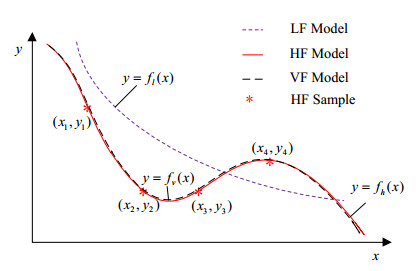
In addition to the above models, some achievements are also made in variable fidelity (VF) approximation models and ensemble approximation models. Variable fidelity model (also termed as multi-fidelity model) is an approximate model constructed by fusion of high and low fidelity samples. In VF model, the global approximation trend of implicit function is reflected by low fidelity model, and the accuracy is guaranteed by introducing a small number of high-fidelity samples ^{[84,85,86,87]}. As shown in Figure 1, the variable fidelity model ${f}_{v}\left(x\right)$ shows good fitting performance to the high-fidelity model ${f}_{h}\left(x\right)$ by fusing the low fidelity model ${f}_{l}\left(x\right)$ and four high fidelity samples.

The VF model is expected to fuse the advantages of LF and HF models and thus become a new choice in engineering. Nevertheless, how to determine the variable fidelity modeling framework and how to quantitatively compare the computational cost of HF model, LF model and VF model still need to be researched ^[88].

Ensemble model is another choice which expects to combines the advantage of multiple single surrogate models ^{[89,90,91,92]}. The modeling strategies of ensemble model can be divided into two categories: weighting and voting ^[90]. The former is based on the prediction accuracy of single models, and a larger weight coefficient is assigned to the model with higher accuracy. The weight coefficients of each single model in the ensemble model is added up to 1 to ensure the accuracy of the prediction value of the ensemble model ^[89,92]. Voting strategy can be regarded as a special weighting strategy, which is usually used in the case of multiple iterations in modeling or optimization. The core is to set the weight of the model with the highest precision to 1, and the weights of other models to 0. In single surrogate models, the modeling performance usually relies on the selection of samples. But the ensemble model can avoid these shortcomings, thus it is able to achieve a robust modeling effect ^[90].

2.2.   Selection of samples

Construction of surrogate model depends on the selection of samples, which can be divided into one-shot sampling methods and sequential sampling methods ^[94]. Commonly used one-shot sampling methods include full factorial design (FFD) ^[94,95], orthogonal design ^[96,97], uniform design ^[98,99], Latin hypercube design (LHD) ^[100,101], etc. Sequential sampling method is to establish the initial surrogate model by one-shot sampling first, and then update the surrogate model by adding samples until the required accuracy is achieved.

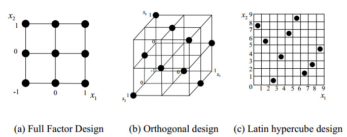
In full factorial design, all levels of each factor are combined to carry out the design of experiments. However, with the increase of design variables and levels, the number of samples required will increase exponentially, which cannot be acceptable in engineering. Therefore, this method is only suitable for the case of fewer design factors and levels. In order to reduce the computational cost of full factorial design, some representative samples instead of all FFD samples can be selected in orthogonal design or uniform design. Furthermore, Latin hypercube design can also be adopted to ensure the representativeness of samples and reduce the repeatability of samples through the layered treatment in the whole design space. Figure 2 shows the sample distribution of 2-factor-3-level full factor experiment design (9 samples), 3-factor-3-level orthogonal experiment design (9 samples) and 9-point Latin hypercube design.

2.3.   Sequential sampling

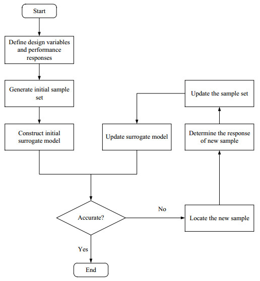
One-shot sampling methods is easy to implement, but the accuracy of the surrogate model cannot be guaranteed. Increasing the number of samples will increase the computational cost and even may cause overfitting. On the contrary, fewer samples will affect the accuracy of surrogate model. Therefore, it is necessary to add sequential samples to update the surrogate model in reliability analysis and RBDO. Sequential sampling methods is a strategy which improves the model accuracy by dividing the modeling process into several stages. The flowchart of sequential sampling methods is shown in Figure 3. First, the initial surrogate model is built by one-shot sampling, and then the surrogate model is updated by adding samples according to some criteria until the required accuracy is achieved.

Figure 4 further describes the process of sequential sampling. $f\left(x\right)$ is the true performance function which needs to be approximated. ${f}_{0}\widehat{(}x)$ is the initial surrogate model constructed by initial samples (black circles) generated from one-shot sampling method. Using the sequential samples (black boxes) to update the surrogate model, the final surrogate mode ${f}_{s}\widehat{(}x)$ with high approximating accuracy is acquired.

The selection of sequential samples can be divided into following methods: error-based methods, methods based on distance to existing samples and methods of sampling near constrained boundaries (Seen in Table 2). The error-based methods can guarantee the accuracy of the surrogate model, but it is difficult to accurately evaluate the modeling error with limit samples. The method based on the distance to the existing samples can evenly distribute the sample points in the design domain. But for highly nonlinear or discontinuous problems, these methods may have poor performance. Sampling near the constraint boundary can improve the fitting accuracy of the constraint boundary, but if the constraint boundary is approximated inaccurately, many samples will be wasted. In engineering, these three sampling methods are often combined to obtain the comprehensive advantages ^{[102,103,104,105]}.

2.4.   Accuracy evaluation of surrogate model

The accuracy of the surrogate model reflects the fitting degree between the predicted response function and the real response function. The following error indexes can be used in accuracy evaluation of surrogate model ^[116]:

(1) Multiple correlation coefficient ${R}^{2}$

${R}^{2}$ is used to evaluate the relative error of the surrogate model in the whole design space ^[117]. The larger the value of ${R}^{2}$, the higher the accuracy of the surrogate model is.

(2) Relative Average Absolute Error (RAAE)

$RAAE$ is used to evaluate the global relative error of the surrogate model. The smaller the value of $RAAE$, the smaller the global relative error is.

(3) Root Mean Squared Error (RMSE)

RMSE is used to evaluate the closeness between the predicted value and the true value ^[118]. The smaller the value of RMSE, the higher the accuracy of the surrogate model is.

(4) Relative Root Mean Squared Error (RRMSE)

RRMSE is used to indicate the degree of accuracy improvement of the surrogate model. The smaller the value of $RRMSE$, the higher the degree of accuracy improvement of the surrogate model is.

(5) Relative Maximum Absolute Error (RMAE)

RMAE is used to evaluate the local prediction error of the surrogate model. The smaller the RMAE value, the smaller the local prediction error of the surrogate model is.

(6) Generalized Mean Square Cross-validation Error ($GMSE$)

GMSE is used to evaluate the prediction error of the surrogate model with limited samples. The smaller the value of $GMSE$, the smaller the prediction error of the surrogate model is.

In equations (9)-(14), $m$ is the number of samples used for model accuracy evaluation; ${y}_{i}$ is the actual response value of performance function, and $\widehat{y}$ is the predicted value obtained by the surrogate model; $\bar y = \frac{1}{m}\sum\limits_{{y_i}}^m {y{}_i}$; ${{\widehat{f}}_{j}}^{\left(-j\right)}$ is the predicted value at point ${x}^{\left(j\right)}$ by the surrogate model constructed using the remaining$m-1$sample points except point $\left({x}^{\left(j\right)}, {f}_{j}\right)$. $MSE$ is the mean square error of the experimental data, $Var$ is the variance of the experimental data, and $STD$ is the standard deviation of the experimental data. $MSE$, $Var$ and $STD$ are calculated as follows:

3.   Surrogate-assisted RBDO methods

In recent decades, many researches have been performed in surrogate-assisted RBDO methods, especially in sequential sampling based RBDO methods. The sequential sampling methods for surrogate model are reviewed in previous section. Different from the sequential sampling methods in surrogate model, some characteristics of RBDO solution process are considered. For example, sequential sampling methods on improving the accuracy of failure probability calculation ^[103,119], using MPP for sequential sampling ^[120], using the samples in the key area of reliability analysis or RBDO ^[122] and using MCS samples to build surrogate model ^[22] are also considered in surrogate-assisted RBDO.

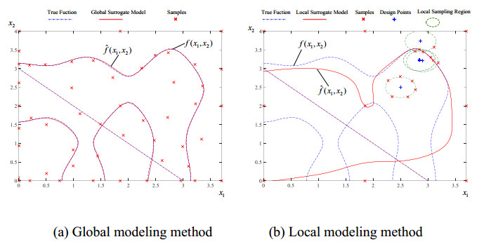
The sequential sampling methods in surrogate-assisted RBDO can be divided into global modeling methods and local modeling methods. It's worth noting that, the global modeling methods can be used in RBDO or other optimization problems, but the local modeling methods can only be used in RBDO. In global modeling methods, accurate performance function boundaries are first approximated in the whole design space (Figure 5(a)), and then RBDO is conducted to find the optimal design. Instead, accurate fitting is only needed in the key area of RBDO (usually near the iterative design point) in local modeling methods (Figure 5(b)). The core of local modeling methods is to update the surrogate model and carry out the design optimization sequentially, as shown in Figure 5 (b) ^[102].

The sample distribution of global modeling methods and local modeling methods are compared in Figure 5. The dotted line is the real performance function curve $f({x}_{1}, {x}_{2})$; the solid line is the prediction curve of the surrogate model $\widehat{f}({x}_{1}, {x}_{2})$; the red "*" is the sample used to construct the surrogate model, and the blue "+" is the optimization iterative design point of RBDO; the green ellipse in Figure 5 (b) is the local sampling region. It can be seen that the global modeling methods fit the boundary of the whole performance function accurately, while the local modeling methods only fit the key area of the optimization iteration.

3.1.   RBDO methods based on global modeling

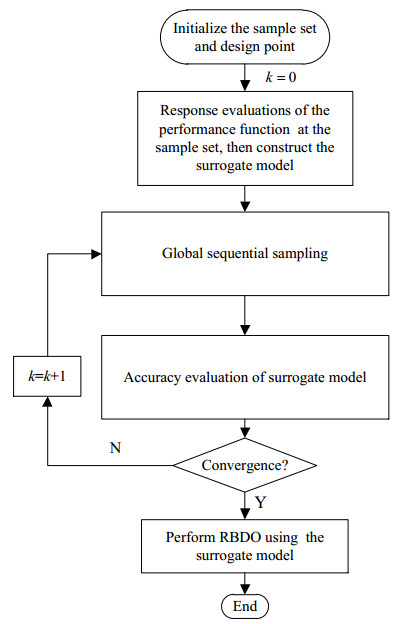
The global modeling methods in RBDO can be divided into the global modeling methods based on one-shot sampling and the global modeling methods based on sequential sampling. Using one-shot sampling, it is difficult to balance the solution precision and computational cost, so current global modeling methods are mostly based on sequential sampling. The basic flowchart of global modeling method in RBDO is shown in Figure 6. After the initial sample set and design point are determined, the initial surrogate model is constructed. And then the surrogate model is updated by global sequential sampling until the accuracy satisfies the requirement. After that, the accurate global surrogate model is used to replace the implicit objective function and performance function in RBDO. Finally, the RBDO problem is solved by double loop methods, single loop methods or decoupling methods.

Following describes the commonly used global modeling methods: Constraint boundary sampling (CBS). Constraint boundary sampling is developed to realize the accurate approximation of the constraint boundary in the whole design space ^[113]. New samples are mainly selected on the approximate constraint boundary. When the accuracy of the global surrogate model satisfies the requirement, RBDO is carried out. The sequential sampling criteria in CBS are as follows:

In CBS, samples locating near the predicted constrained boundary will be preferred.

3.2.   RBDO method based on local modeling

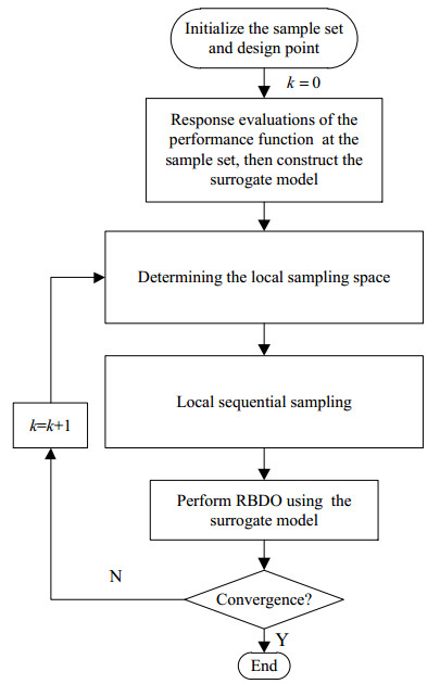
The global modeling method can fit the constraint boundary in the whole design space well, but there are always some inactive samples in RBDO (Such as the samples located on the lower left quarter in Figure 5(a)), which will inevitably cause waste of computational resources. Therefore, the local modeling methods to fit the key region of design space is proposed. The flowchart of local modeling methods is shown in Figure 7. Different from global sampling methods, the sequential samples are mainly selected in a small local region around the current design which is calculated by double loop methods, single loop methods or decoupling methods. Therefore, the RBDO process and sequential sampling are conducted sequentially.

Following is a brief introduction of the representative local modeling method LAS (local adaptive sampling method). In LAS, the samples are preferentially selected near the constraint boundaries around the current design point ^[102]. The size of local sampling region is determined according to the target reliability and nonlinearity of the performance functions, which is shown as:

Where $nc$ is used to quantify the nonlinearity of the performance functions; ${\mathit \nabla } {\widehat{g}}_{i}\left(x\right)$ is the predicted gradient value at $x$ for the ith probabilistic constraint. $\left({x}^{1}, \cdots, {x}^{M}\right)$ are the M testing points evenly located within the ${\beta }^{t}$-sphere region. $N$is the number of probabilistic constraints. Seen from Eq. (17), a larger local sampling region is assigned to performance function with larger target reliability and higher nonlinearity.

After the local sampling region is determined, MSE sampling criterion and CBS criterion are introduced to select the sequential samples. The detailed sequential sampling criterion in LAS is as follows:

In Eq. (18), if no performance function boundary is contained in the local sampling region, the prediction error and distance to the existing samples are used to select new samples. Otherwise, CBS sampling criterion in Eq. (16) is adopted.

3.3.   Numerical example

To compare the performance of global modeling method and local modeling method, a two-dimensional RBDO problem with three probabilistic constraints is introduced, which is formulated as follows:

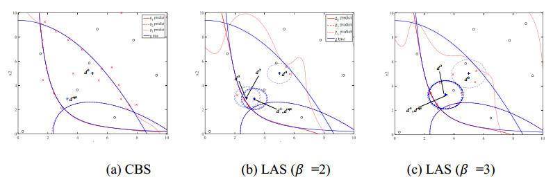
Figure 8 shows the locations of sample points when using CBS and LAS to solve this problem. Black "o" is the initial samples using LHS method and red "x" is the sequential samples; blue "+" is the design point. ${d}^{0}$ is the initial design point and ${d}^{opt}$ is the optimal design point. As can be seen, both the CBS method and LAS method can obtain the optimal design ${d}^{opt}$. The surrogate model using CBS method has good fit performance in the whole design space and most sequential sample points are located near the constraint boundary (Seen in Figure 8(a)). Differently, most of the sequential sample points in LAS are concentrated in the small local region around current iterative design points (Blue ellipse in Figure 8(b)). Therefore, the fitting capability of surrogate model is weak in the upper right quarter of the design space. Because sequential sampling is avoided in the meaningless region of RBDO process, LAS has higher efficiency. It's worth noting that, if the target reliability changes, the sequential sampling process of LAS method will be conducted again. Therefore, the surrogate model constructed by LAS cannot be reused (Seen in Figure 8(c)).

Table 3 shows the comparison of global modeling methods and local modeling methods. In global modeling methods, an accurate global surrogate model is built in the whole design space, therefore this model can also be used when the target reliability changes. But when the target reliability is fixed, the efficiency is usually lower than local modeling methods (Seen in Figure 8). On the other hand, the local modeling method is more efficient for problem with fixed target reliability. But when the target reliability changes, the local sampling region and corresponding sequential sample points will change, which means different surrogate models must be built for problems with different target reliability.

4.   Summary and prospect

In this paper, the surrogate-assisted RBDO methods are reviewed. Commonly used reliability analysis methods, RBDO methods, surrogate models and corresponding sampling and accuracy evaluation methods are summarized and discussed. Then the surrogate-assisted RBDO methods are divided into the global modeling methods and local modeling methods. The advantages and dis advantages of these two methods are compared.

(1) This paper introduces the mathematical model of RBDO, summarizes the existing reliability analysis methods and RBDO methods. Different RBDO methods are classified and compared.

(2) This paper summarizes the commonly used surrogate model, sampling method and accuracy evaluation methods of surrogate models. Different sampling methods are classified and compared.

(3) This paper divided the surrogate-assisted RBDO methods into the global modeling methods and local modeling methods. Using a representative numerical example, the advantages and disadvantages of these two modeling methods are compared.

Although many surrogate-assisted RBDO methods have been developed, there are still some research space to further strengthen the application of these methods in engineering. Future researches can be focused on the following aspects:

(1) Quantification of modeling error of surrogate model

Generally, the number of samples used to build the surrogate model is finite, thus the prediction accuracy of the surrogate model cannot be well guaranteed. Meanwhile, in existing researches, the modeling error of surrogate model is mainly used in sequential sampling. This strategy can achieve the optimal RBDO solution for general functions, but it may have large error for multimodal functions, or even cannot meet the reliability requirements. Therefore, it is of great significance to quantify the modeling error and construct its conservative model as an alternative to the implicit performance function, which finally achieve the performance improvement on the premise of ensuring the reliability requirements.

(2) Determination of high-fidelity samples and low fidelity samples in variable fidelity model

Commonly used variable fidelity methods are based on the situation that the function form (often from empirical formula, etc.) of the low fidelity model is known. In view of the unknown function form of low fidelity model, it is very important to allocate the high and low fidelity samples reasonably in RBDO process. In addition, the study of the variable fidelity method based on the surrogate model will also be a useful supplement.

(3) Construction of surrogate model for high dimensional RBDO problem with limited samples

The existence of "dimension disaster" makes the computational cost of existing RBDO methods unacceptable, which not only exists in the construction of surrogate model, but also in the process of reliability analysis and design optimization. In order to acquire an accurate and efficient RBDO solution, the problem dimension must be limited. Effective variable selection methods, high dimensional model representation methods, high dimensional reliability analysis methods and high dimensional optimization methods will be future research hotspots.

(4) Construction of classification model to balance the precision and cost in RBDO

Besides using surrogate models to accurately approximate the implicit objective and performance functions, introduction of the classification method such as support vector machine is another viable option. However, the existing support vector machine method is commonly confronted with precision problem because of lack of real function response information. Therefore, it is necessary to develop a more effective classification model to balance the precision and cost in RBDO.

Acknowledgments

This research was funded by National Natural Science Foundation of China (Grant No. 51905492), Key Scientific and Technological Research Projects in Henan Province (Grant No. 202102210089, 202102210274), Innovative Research Team (in Science and Technology) in University of Henan Province (Grant No. 20IRTSTHN015).