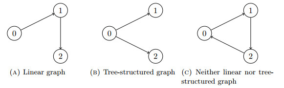
In this paper, we consider a stationary model for the flow through a network. The flow is determined by the values at the boundary nodes of the network. We call these values the loads of the network. In the applications, the feasible loads must satisfy some box constraints. We analyze the structure of the set of feasible loads. Our analysis is motivated by gas pipeline flows, where the box constraints are pressure bounds.
We present sufficient conditions that imply that the feasible set is star-shaped with respect to special points. Under stronger conditions, we prove the convexity of the set of feasible loads. All the results are given for passive networks with and without compressor stations.
This analysis is motivated by the aim to use the spheric-radial decomposition for stochastic boundary data in this model. This paper can be used for simplifying the algorithmic use of the spheric-radial decomposition.
Citation: Martin Gugat, Rüdiger Schultz, Michael Schuster. Convexity and starshapedness of feasible sets in stationary flow networks[J]. Networks and Heterogeneous Media, 2020, 15(2): 171-195. doi: 10.3934/nhm.2020008
In this paper, we consider a stationary model for the flow through a network. The flow is determined by the values at the boundary nodes of the network. We call these values the loads of the network. In the applications, the feasible loads must satisfy some box constraints. We analyze the structure of the set of feasible loads. Our analysis is motivated by gas pipeline flows, where the box constraints are pressure bounds.
We present sufficient conditions that imply that the feasible set is star-shaped with respect to special points. Under stronger conditions, we prove the convexity of the set of feasible loads. All the results are given for passive networks with and without compressor stations.
This analysis is motivated by the aim to use the spheric-radial decomposition for stochastic boundary data in this model. This paper can be used for simplifying the algorithmic use of the spheric-radial decomposition.

| [1] |
Coupling conditions for gas networks governed by the isothermal Euler equations. Netw. Heterog. Media (2006) 1: 295-314. 
|
| [2] |
Gas flow in pipeline networks. Netw. Heterog. Media (2006) 1: 41-56.
|
| [3] | Simulation and optimization models of steady-state gas transmission networks. Energy Procedia (2015) 64: 130-139. |
| [4] |
Euler systems for compressible fluids at a junction. J. Hyperbolic Differ. Equ. (2008) 5: 547-568.
|
| [5] | P. Domschke, B. Hiller, J. Lang and C. Tischendorf, Modellierung von Gasnetzwerken: Eine Übersicht, (2019), Preprint on Webpage http://tubiblio.ulb.tu-darmstadt.de/106763/. |
| [6] |
Properties of chance constraints in infinite dimensions with an application to PDE constrained optimization. Set-Valued Var. Anal. (2018) 26: 821-841.
|
| [7] |
A. Genz and F. Bretz, Computation of Multivariate Normal and $t$ Probabilities, Lecture Notes in Statistics, 195. Springer, Dordrecht, 2009. doi: 10.1007/978-3-642-01689-9
|
| [8] |
A joint model of probabilistic/robust constraints for gas transport management in stationary networks. Comput. Manag. Sci. (2017) 14: 443-460.
|
| [9] |
On the quantification of nomination feasibility in stationary gas networks with random load. Math. Methods Oper. Res. (2016) 84: 427-457.
|
| [10] |
Stationary states in gas networks. Netw. Heterog. Media (2015) 10: 295-320.
|
| [11] |
Networks of pipelines for gas with nonconstant compressibility factor: Stationary states. J. Comput. Appl. Math. (2018) 37: 1066-1097.
|
| [12] |
M. Gugat and M. Schuster, Stationary gas networks with compressor control and random loads: Optimization with probabilistic constraints, Math. Probl. Eng., 2018 (2018), Art. ID 7984079, 17 pp. doi: 10.1155/2018/7984079
|
| [13] |
The isothermal Euler equations for ideal gas with source term: Product solutions, flow reversal and no blow up. J. Math. Anal. Appl. (2017) 454: 439-452.
|
| [14] |
Transient flow in gas networks: Traveling waves. Int. J. Appl. Math. Comput. Sci. (2018) 28: 341-348.
|
| [15] |
H. Heitsch, On probabilistic capacity maximization in a stationary gas network, Optimization, 69 (2020), 575–604, Preprint on Webpage http://wias-berlin.de/publications/wias-publ/run.jsp?template=abstract&type=Preprint&year=2018&number=2540. doi: 10.1080/02331934.2019.1625353
|
| [16] |
T. Koch, B. Hiller, M. E. Pfetsch and L. Schewe, Evaluating Gas Network Capacities, MOS-SIAM Series on Optimization, 21. Society for Industrial and Applied Mathematics (SIAM), Philadelphia, PA, 2015. doi: 978-1-611973-68-6
|
| [17] |
A. Prékopa, Stochastic Programming, Mathematics and its Applications, 324. Kluwer Academic Publishers Group, Dordrecht, 1995. doi: 10.1007/978-94-017-3087-7
|
| [18] |
Computational optimization of gas compressor stations: MINLP models versus continuous reformulations. Math. Methods Oper. Res. (2016) 83: 409-444.
|
| [19] |
Extensions of stochastic optimization results to problems with system failure probability functions. J. Optim. Theory Appl. (2007) 133: 1-18.
|
| [20] |
L. Schewe, M. Schmidt and J. Thürauf, Structural properties of feasible bookings in the European entry-exit gas market system, 4OR, (2019). doi: 10.1007/s10288-019-00411-3
|
| [21] |
(Sub-)Differentiability of probabilistic functions with elliptical distributions. Set-Valued Var. Anal. (2018) 26: 887-910.
|
| [22] |
Gradient formulae for nonlinear probabilistic constraints with Gaussian and Gaussian-like distribution. SIAM J. Optim. (2014) 24: 1864-1889.
|
| [23] | D. Wintergerst, Application of chance constrained optimization to gas networks, (2019), Preprint on Webpage https://opus4.kobv.de/opus4-trr154/frontdoor/index/index/start/5/rows/10/sortfield/score/sortorder/desc/searchtype/simple/query/wintergerst/docId/158. |


Figures(16)
Martin Gugat, Rüdiger Schultz, Michael Schuster. Convexity and starshapedness of feasible sets in stationary flow networks[J]. Networks and Heterogeneous Media, 2020, 15(2): 171-195. doi: 10.3934/nhm.2020008


 DownLoad: