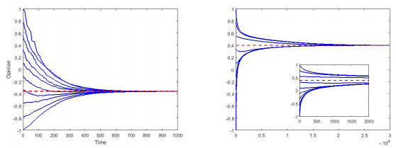
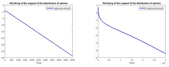
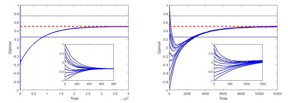
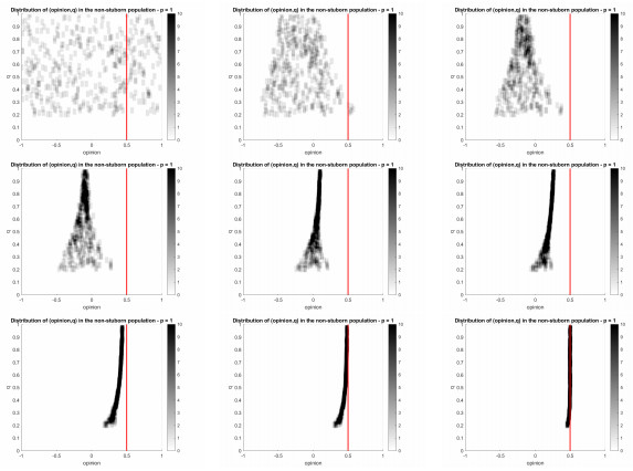
In this work we study the formation of consensus in homogeneous and heterogeneous populations, and the effect of attractiveness or fitness of the opinions. We derive the corresponding kinetic equations, analyze the long time behavior of their solutions, and characterize the consensus opinion.
Citation: Mayte Pérez-Llanos, Juan Pablo Pinasco, Nicolas Saintier. Opinion fitness and convergence to consensus in homogeneous and heterogeneous populations[J]. Networks and Heterogeneous Media, 2021, 16(2): 257-281. doi: 10.3934/nhm.2021006
In this work we study the formation of consensus in homogeneous and heterogeneous populations, and the effect of attractiveness or fitness of the opinions. We derive the corresponding kinetic equations, analyze the long time behavior of their solutions, and characterize the consensus opinion.

| [1] |
G. Aletti, A. K. Naimzada and G. Naldi., Mathematics and physics applications in sociodynamics simulation: The case of opinion formation and diffusion, Mathematical Modeling of Collective Behavior in Socio-Economic and Life Sciences, Birkhäuser Boston, (2010), 203–221. doi: 10.1007/978-0-8176-4946-3_8

|
| [2] |
First-order continuous models of opinion formation. SIAM J. Appl. Math. (2007) 67: 837-853.
|
| [3] |
Opinions and social pressure. Scientific American (1955) 193: 31-35.
|
| [4] | R. B. Ash, Real Analysis and Probability, Probability and Mathematical Statistics, Academic Press, New York-London, 1972. |
| [5] | P. Balenzuela, J. P. Pinasco and V. Semeshenko, The undecided have the key: Interaction driven opinion dynamics in a three state model, PLoS ONE, 10 (2016), e0139572, 1–21. |
| [6] |
Opinion strength influences the spatial dynamics of opinion formation. The Journal of Mathematical Sociology (2016) 40: 207-218.
|
| [7] | B. O. Baumgaertner, P. A. Fetros, R. C. Tyson and S. M. Krone, Spatial Opinion Dynamics and the Efects of Two Types of Mixing, Phys Rev E., 98 (2018), 022310. |
| [8] | N. Bellomo, Modeling Complex Living Systems A Kinetic Theory and Stochastic Game Approach, Birkhauser, 2008. |
| [9] |
N. Bellomo, G. Ajmone Marsan and A. Tosin, Complex Systems and Society. Modeling and Simulation, SpringerBriefs in Mathematics, 2013. doi: 10.1007/978-1-4614-7242-1
|
| [10] | K. C. Border and C. D. Aliprantis, Infinite Dimensional Analysis - A Hitchhiker's Guide, 3rd Edition, Springer, 2006. |
| [11] |
What a person thinks upon learning he has chosen differently from others: Nice evidence for the persuasive-arguments explanation of choice shifts. Journal of Experimental Social Psychology (1975) 11: 412-426.
|
| [12] |
A well-posedness theory in measures for some kinetic models of collective motion. Mathematical Models and Methods in Applied Sciences (2011) 21: 515-539.
|
| [13] | R. B. Cialdini and M. R. Trost, Social influence: Social norms, conformity and compliance, The Handbook of Social Psychology, McGraw-Hill, (1998), 151–192. |
| [14] |
Emergent behavior in flocks. IEEE Transactions on Automatic Control (2007) 52: 852-862.
|
| [15] |
Mixing beliefs among interacting agents. Advances in Complex Systems (2000) 3: 87-98.
|
| [16] |
A note on generalized inverse. Mathematical Methods of Operations Research (2013) 77: 423-432.
|
| [17] |
Social influence and opinions. Journal of Mathematical Sociology (1990) 15: 193-206.
|
| [18] | A simple model of consensus formation. Okayama Economic Review (1999) 31: 95-100. |
| [19] |
S. Galam, Sociophysics: A Physicist's Modeling of Psycho-Political Phenomena, , Springer Science & Business Media, 2012. doi: 10.1007/978-1-4614-2032-3
|
| [20] | R. Hegselmann and U. Krause, Opinion dynamics and bounded confidence: Models, analysis and simulation, Journal of Artificial Societies and Social Simulation, 5 (2002). |
| [21] |
Ergodic theorems for weakly interacting infinite systems and the voter model. The Annals of Probability (1975) 3: 643-663.
|
| [22] |
C. La Rocca, L. A. Braunstein and F. Vázquez, The influence of persuasion in opinion formation and polarization, Europhys. Letters, 106 (2014), 40004. doi: 10.1209/0295-5075/106/40004
|
| [23] | The psychology of social impact. American Psychologist (1981) 36: 343-356. |
| [24] |
Continuous opinion dynamics under bounded confidence: A survey. International Journal of Modern Physics C (2007) 18: 1819-1838.
|
| [25] | M. Mäs and A. Flache, Differentiation without distancing. Explaining bi-polarization of opinions without negative influence, PloS one, 8 (2013), e74516. |
| [26] |
Envelope theorems for arbitrary choice sets. Econometrica (2002) 70: 583-601.
|
| [27] |
Simulation of Sznajd sociophysics model with convincing single opinions. International Journal of Modern Physics C (2001) 12: 1091-1092.
|
| [28] | (2014) Interacting Multiagent Systems: Kinetic Equations and Monte Carlo Methods. Oxford: Oxford University Press. |
| [29] |
Measure-valued opinion dynamics. M3AS: Mathematical Models and Methods in Applied Sciences (2020) 30: 225-260.
|
| [30] |
M. Pérez-Llanos, J. P. Pinasco and N. Saintier, Opinion attractiveness and its effect in opinion formation models, Phys. A, 559 (2020), 125017, 9 pp. doi: 10.1016/j.physa.2020.125017
|
| [31] |
Opinion formation models with heterogeneous persuasion and zealotry. SIAM Journal on Mathematical Analysis (2018) 50: 4812-4837.
|
| [32] | F. Vazquez, N. Saintier and J. P. Pinasco, The role of voting intention in public opinion polarization, Phys. Rev. E, 101 (2020), 012101, 13pp. |
| [33] |
N. Saintier, J. P. Pinasco and F. Vazquez, A model for a phase transition between political mono-polarization and bi-polarization, Chaos: An Interdisciplinary Journal of Nonlinear Science, 30 (2020), 063146, 17 pp. doi: 10.1063/5.0004996
|
| [34] |
Modeling opinion dynamics: Theoretical analysis and continuous approximation. Chaos, Solitons & Fractals (2017) 98: 210-215.
|
| [35] |
F. Slanina and H. Lavicka, Analytical results for the Sznajd model of opinion formation, The European Physical Journal B, 35 (2003) 279–288. doi: 10.1140/epjb/e2003-00278-0
|
| [36] | (1993) Probability Theory, An Analytic View. Cambridge University Press. |
| [37] |
Opinion evolution in closed community. International Journal of Modern Physics - C (2000) 11: 1157-1165.
|
| [38] |
Kinetic models of opinion formation. Communications in Mathematical Sciences (2006) 4: 481-496.
|
| [39] |
C. Villani, Topics in optimal transportation, Grad.Studies in Math., American Mathematical Soc., (2003). doi: 10.1090/gsm/058
|
Figures(4)
Mayte Pérez-Llanos, Juan Pablo Pinasco, Nicolas Saintier. Opinion fitness and convergence to consensus in homogeneous and heterogeneous populations[J]. Networks and Heterogeneous Media, 2021, 16(2): 257-281. doi: 10.3934/nhm.2021006


 DownLoad: