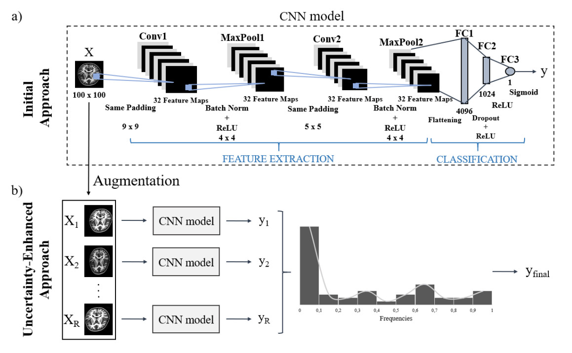
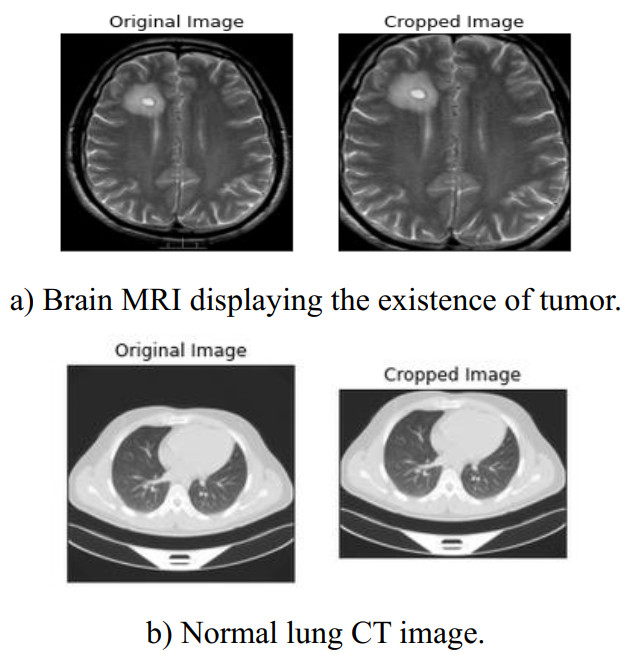
The automated detection of tumors using medical imaging data has garnered significant attention over the past decade due to the critical need for early and accurate diagnoses. This interest is fueled by advancements in computationally efficient modeling techniques and enhanced data storage capabilities. However, methodologies that account for the uncertainty of predictions remain relatively uncommon in medical imaging. Uncertainty quantification (UQ) is important as it helps decision-makers gauge their confidence in predictions and consider variability in the model inputs. Numerous deterministic deep learning (DL) methods have been developed to serve as reliable medical imaging tools, with convolutional neural networks (CNNs) being the most widely used approach. In this paper, we introduce a low-complexity uncertainty-based CNN architecture for medical image classification, particularly focused on tumor and heart failure (HF) detection. The model's predictive (aleatoric) uncertainty is quantified through a test-set augmentation technique, which generates multiple surrogates of each test image. This process enables the construction of empirical distributions for each image, which allows for the calculation of mean estimates and credible intervals. Importantly, this methodology not only provides UQ, but also significantly improves the model's classification performance. This paper represents the first effort to demonstrate that test-set augmentation can significantly improve the classification performance of medical images. The proposed DL model was evaluated using three datasets: (a) brain magnetic resonance imaging (MRI), (b) lung computed tomography (CT) scans, and (c) cardiac MRI. The low-complexity design of the model enhances its robustness against overfitting, while it is also easily re-trainable in case out-of-distribution data is encountered, due to the reduced computational resources required by the introduced architecture.
Citation: Vasileios E. Papageorgiou, Georgios Petmezas, Pantelis Dogoulis, Maxime Cordy, Nicos Maglaveras. Uncertainty CNNs: A path to enhanced medical image classification performance[J]. Mathematical Biosciences and Engineering, 2025, 22(3): 528-553. doi: 10.3934/mbe.2025020
The automated detection of tumors using medical imaging data has garnered significant attention over the past decade due to the critical need for early and accurate diagnoses. This interest is fueled by advancements in computationally efficient modeling techniques and enhanced data storage capabilities. However, methodologies that account for the uncertainty of predictions remain relatively uncommon in medical imaging. Uncertainty quantification (UQ) is important as it helps decision-makers gauge their confidence in predictions and consider variability in the model inputs. Numerous deterministic deep learning (DL) methods have been developed to serve as reliable medical imaging tools, with convolutional neural networks (CNNs) being the most widely used approach. In this paper, we introduce a low-complexity uncertainty-based CNN architecture for medical image classification, particularly focused on tumor and heart failure (HF) detection. The model's predictive (aleatoric) uncertainty is quantified through a test-set augmentation technique, which generates multiple surrogates of each test image. This process enables the construction of empirical distributions for each image, which allows for the calculation of mean estimates and credible intervals. Importantly, this methodology not only provides UQ, but also significantly improves the model's classification performance. This paper represents the first effort to demonstrate that test-set augmentation can significantly improve the classification performance of medical images. The proposed DL model was evaluated using three datasets: (a) brain magnetic resonance imaging (MRI), (b) lung computed tomography (CT) scans, and (c) cardiac MRI. The low-complexity design of the model enhances its robustness against overfitting, while it is also easily re-trainable in case out-of-distribution data is encountered, due to the reduced computational resources required by the introduced architecture.

| [1] | S. A. Alowais, S. S. Alghamdi, N. Alsuhebany, T. Alqahtani, A. I. Alshaya, S. N. Almohareb, et al., Revolutionizing healthcare: The role of artificial intelligence in clinical practice, BMC Med. Educ., 23 (2023), 689. |
| [2] |
D. Saligkaras, V. E. Papageorgiou, On the detection of patterns in electricity prices across European countries: An unsupervised machine learning approach, AIMS Energy, 10 (2022), 1146–1164. https://doi.org/10.3934/energy.2022054 doi: 10.3934/energy.2022054

|
| [3] |
D. Saligkaras, V. E. Papageorgiou, Seeking the truth beyond the data. An unsupervised machine learning approach, AIP Conf. Proc., 2812 (2023), 020106. https://doi.org/10.1063/5.0161454 doi: 10.1063/5.0161454
|
| [4] |
S. S. Kshatri, D. Singh, Convolutional neural network in medical image analysis: A review, Arch. Comput. Methods Eng., 30 (2023), 2793–2810. https://doi.org/10.1007/s11831-023-09898-w doi: 10.1007/s11831-023-09898-w
|
| [5] |
K. Zou, Z. Chen, X. Yuan, X. Shen, M. Wang, H. Fu, A review of uncertainty estimation and its application in medical imaging, Meta-Radiol., 1 (2023), 100003. https://doi.org/10.1016/j.metrad.2023.100003 doi: 10.1016/j.metrad.2023.100003
|
| [6] |
L. Huang, S. Ruan, Y. Xing, M. Feng, A review of uncertainty quantification in medical image analysis: Probabilistic and non-probabilistic methods, Med. Image Anal., 97 (2024), 103223. https://doi.org/10.1016/j.media.2024.103223 doi: 10.1016/j.media.2024.103223
|
| [7] |
M. M. Jassim, Systematic review for lung cancer detection and lung nodule classification: Taxonomy, challenges, and recommendation future works, J. Intell. Syst., 31 (2022), 944–964. https://doi.org/10.1515/jisys-2022-0062 doi: 10.1515/jisys-2022-0062
|
| [8] |
H. Sung, J. Ferlay, R. L. Siegel, M. Laversanne, I. Soerjomataram, A. Jemal, et al., Global cancer statistics 2020: GLOBOCAN estimates of incidence and mortality worldwide for 36 cancers in 185 countries, CA Cancer J. Clin., 71 (2021), 209–249. https://doi.org/10.3322/caac.21660 doi: 10.3322/caac.21660
|
| [9] |
G. Savarese, P. M. Becher, L. H. Lund, P. Seferovic, G. M. C. Rosano, A. J. S. Coats, Global burden of heart failure: A comprehensive and updated review of epidemiology, Cardiovasc. Res., 119 (2023), 1453. https://doi.org/10.1093/cvr/cvad026 doi: 10.1093/cvr/cvad026
|
| [10] |
A. Inamdar, A. Inamdar, Heart failure: Diagnosis, management and utilization, J. Clin. Med., 5 (2016), 62. https://doi.org/10.3390/jcm5070062 doi: 10.3390/jcm5070062
|
| [11] |
L. Li, J. Chang, A. Vakanski, Y. Wang, T. Yao, M. Xian, Uncertainty quantification in multivariable regression for material property prediction with Bayesian neural networks, Sci. Rep., 14 (2024), 1783. https://doi.org/10.1038/s41598-024-61189-x doi: 10.1038/s41598-024-61189-x
|
| [12] |
A. Olivier, M. D. Shields, L. Graham-Brady, Bayesian neural networks for uncertainty quantification in data-driven materials modeling, Comput. Methods Appl. Mech. Eng., 386 (2021), 114079. https://doi.org/10.1016/j.cma.2021.114079 doi: 10.1016/j.cma.2021.114079
|
| [13] |
M. Malmström, I. Skog, D. Axehill, F. Gustafsson, Uncertainty quantification in neural network classifiers—A local linear approach, Automatica, 163 (2024), 111563. https://doi.org/10.1016/j.automatica.2024.111563 doi: 10.1016/j.automatica.2024.111563
|
| [14] | A. Kendall, Y. Gal, What uncertainties do we need in Bayesian deep learning for computer vision?, Adv. Neural Inf. Process. Syst., 30 (2017). |
| [15] |
J. Gawlikowski, C. R. N. Tassi, M. Ali, J. Lee, M. Humt, J. Feng, et al., A survey of uncertainty in deep neural networks, Artif. Intell. Rev., 56 (2023), 1513–1589. https://doi.org/10.1007/s10462-023-10562-9 doi: 10.1007/s10462-023-10562-9
|
| [16] | B. Lakshminarayanan, A. Pritzel, C. Blundell, Simple and scalable predictive uncertainty estimation using deep ensembles, Adv. Neural Inf. Process. Syst., 31 (2017), 6405–6416. |
| [17] |
A. R. Tan, S. Urata, S. Goldman, J. C. B. Dietschreit, R. Gómez-Bombarelli, Single-model uncertainty quantification in neural network potentials does not consistently outperform model ensembles, npj Comput. Mater., 9 (2023), 148. https://doi.org/10.1038/s41524-023-01180-8 doi: 10.1038/s41524-023-01180-8
|
| [18] |
G. Gao, H. Jiang, J. C. Vink, C. Chen, Y. El Khamra, J. J. Ita, Gaussian mixture model fitting method for uncertainty quantification by conditioning to production data, Comput. Geosci., 24 (2019), 663–681. https://doi.org/10.1007/s10596-019-9823-3 doi: 10.1007/s10596-019-9823-3
|
| [19] | S. Manjunath, M. B. S. Pande, B. N. Raveesh, G. K. Madhusudhan, Brain tumor detection and classification using convolution neural network, Int. J. Recent Technol. Eng., 8 (2019), 34–40. |
| [20] | R. H. Ramdlon, E. M. Kusumaningtyas, T. Karlita, Brain tumor classification using MRI images with K-nearest neighbor method, 2019 Int. Electron. Symp., (2019), 660–667. https://doi.org/10.1109/ELECSYM.2019.8901560 |
| [21] | N. Vani, A. Sowmya, N. Jayamma, Brain tumor classification using support vector machine, Int. Res. J. Eng. Technol., 4 (2017), 1724–1729. |
| [22] | A. R. Mathew, P. B. Anto, Tumor detection and classification of MRI brain image using wavelet transform and SVM, in 2017 International Conference on Signal Processing and Communication (ICSPC), (2017). https://doi.org/10.1109/CSPC.2017.8305810 |
| [23] |
J. Seetha, S. S. Raja, Brain tumor classification using convolutional neural networks, Biomed. Pharmacol. J., 11 (2018), 1457–1461. https://dx. doi.org/10.13005/bpj/1511 doi: 10.13005/bpj/1511
|
| [24] | K. R. Babu, U. S. Deepthi, A. S. Madhuri, P. S. Prasad, S. Shammem, Comparative analysis of brain tumor detection using deep learning methods, Int. J. Sci. Technol. Res., 8 (2019), 250–254. |
| [25] | K. Pathak, M. Pavthawala, N. Patel, D. Malek, V. Shah, B. Vaidya, Classification of brain tumor using convolutional neural network, in 2019 3rd International conference on Electronics, Communication and Aerospace Technology (ICECA), (2019), 128–132. https://doi.org/10.1109/ICECA.2019.8821931 |
| [26] |
S. M. Kulkarni, G. Sundari, Brain MRI classification using deep learning algorithm, Int. J. Eng. Adv. Technol., 9 (2020), 1226–1231. https://doi.org/10.35940/ijeat.C5350.029320 doi: 10.35940/ijeat.C5350.029320
|
| [27] | R. Lang, K. Jia, J. Feng, Brain tumor identification based on CNN-SVM model, in Proceedings of the 2nd International Conference on Biomedical Engineering and Bioinformatics, (2018), 31–35. https://doi.org/10.1145/3278198.3278209 |
| [28] |
E. Sert, F. Ӧzyurt, A. Doğanteklin, A new approach for brain tumor diagnosis system: Single image super-resolution-based maximum fuzzy entropy segmentation and convolutional neural network, Med. Hypotheses, 133 (2019), 109438. https://doi.org/10.1016/j.mehy.2019.109413 doi: 10.1016/j.mehy.2019.109413
|
| [29] |
F. Ӧzyurt, E. Sert, E. Avci, E. Doğanteklin, Brain tumor detection on convolutional neural networks with neutrosophic expert maximum fuzzy sure entropy, Measurement, 147 (2019), 106830. https://doi.org/10.1016/j.measurement.2019.07.058 doi: 10.1016/j.measurement.2019.07.058
|
| [30] | P. Saxena, A. Maheshwari, S. Maheshwari, Predictive modeling of brain tumor: A deep learning approach, in Innovations in Computational Intelligence and Computer Vision: Proceedings of ICICV 2020, (2020), 275–285. |
| [31] | S. Das, O. F. M. Riaz, R. Aranya, N. N. Labiba, Brain tumor classification using convolutional neural network, Int. Conf. Adv. Sci. Eng. Robot. Technol., 2019. |
| [32] | P. Afshar, K. N. Plataniotis, A. Mohammadi, Capsule networks for brain tumor classification based on MRI images and coarse tumor boundaries, in ICASSP 2019-2019 IEEE International Conference on Acoustics, Speech and Signal Processing (ICASSP), (2019), 1368–1372. https://doi.org/10.1109/ICASSP.2019.8683759 |
| [33] | A. M. Alqudah, H. Alquraan, I. A. Qasmieh, A. Alqudah, W. Al-Sharu, Brain tumor classification using deep learning technique–A comparison between cropped, uncropped, and segmented lesion images with different sizes, Int. J. Adv. Trends Comput. Sci. Eng., 8 (2019), 3684–3691. |
| [34] | Y. Zhou, Z. Li, H. Zhu, C. Chen, M. Gao, K. Xu, et al., Holistic brain tumor screening and classification based on DenseNet and recurrent neural network, in Brainlesion: Glioma, Multiple Sclerosis, Stroke and Traumatic Brain Injuries: 4th International Workshop, BrainLes 2018, Held in Conjunction with MICCAI 2018, Granada, Spain, September 16, 2018, Revised Selected Papers, Part I 4., 11383 (2019), 208–217. https://doi.org/10.1007/978-3-030-11723-8_21 |
| [35] |
H. F. Kareem, M. S. Al-Husieny, F. Y. Mohsen, E. A. Khalil, Z. S. Hassan, Evaluation of SVM performance in the detection of lung cancer in marked CT scan dataset, Indones. J. Electr. Eng. Comput. Sci., 21 (2021), 1731–1738. http://doi.org/10.11591/ijeecs.v21.i3.pp1731-1738 doi: 10.11591/ijeecs.v21.i3.pp1731-1738
|
| [36] |
M. S. Al-Huseiny, A. S. Sajit, Transfer learning with GoogLeNet for detection of lung cancer, Indones. J. Electr. Eng. Comput. Sci., 22 (2021), 1078–1086. http://doi.org/10.11591/ijeecs.v22.i2.pp1078-1086 doi: 10.11591/ijeecs.v22.i2.pp1078-1086
|
| [37] |
S. M. Naqi, M. Sharif, I. U. Lali, A 3D nodule candidate detection method supported by hybrid features to reduce false positives in lung nodule detection, Multimed. Tools Appl., 78 (2019), 26287–26311. https://doi.org/10.1007/s11042-019-07819-3 doi: 10.1007/s11042-019-07819-3
|
| [38] | W. Abbas, K. B. Khan, M. Aqeel, M. A. Azam, M. H. Ghouri, F. H. Jaskani, Lungs nodule cancer detection using statistical techniques, in 2020 IEEE 23rd International Multitopic Conference (INMIC), (2020), 1–6. https://doi.org/10.1109/INMIC50486.2020.9318181 |
| [39] | K. Roy, S. S. Chaudhury, M. Burman, A. Ganguly, C. Dutta, S. Banik, et al., A comparative study of lung cancer detection using supervised neural network, in 2019 International Conference on Opto-Electronics and Applied Optics (Optronix), (2019), 1–5. https://doi.org/10.1109/OPTRONIX.2019.8862326 |
| [40] | A. Mohite, Application of transfer learning technique for detection and classification of lung cancer using CT images, Int. J. Sci. Res. Manag., 9 (2021), 621–634. |
| [41] |
H. Polat, H. D. Mehr, Classification of pulmonary CT images by using hybrid 3D-deep convolutional neural network architecture, Appl. Sci., 9 (2019), 940. https://doi.org/10.3390/app9050940 doi: 10.3390/app9050940
|
| [42] | S. Mukherjee, S. U. Bohra, Lung cancer disease diagnosis using machine learning approach, in 2020 3rd International Conference on Intelligent Sustainable Systems (ICISS), (2020), 207–211. https://doi.org/10.1109/ICISS49785.2020.9315909 |
| [43] | A. Hoque, A. K. M. A. Farabi, F. Ahmed, M. Z. Islam, Automated detection of lung cancer using CT scan images, in 2020 IEEE Region 10 Symposium (TENSYMP), (2020), 1030–1033. https://doi.org/10.1109/TENSYMP50017.2020.9230861 |
| [44] |
G. Petmezas, V. E. Papageorgiou, V. Vassilikos, E. Pagourelias, G. Tsaklidis, A. K. Katsaggelos, et al., Recent advancements and applications of deep learning in heart failure: A systematic review, Comput. Biol. Med., 176 (2024), 108557. https://doi.org/10.1016/j.compbiomed.2024.108557 doi: 10.1016/j.compbiomed.2024.108557
|
| [45] | J. M. Wolterink, T. Leiner, M. A. Viergever, I. Išgum, Automatic segmentation and disease classification using cardiac cine MR images, Lect. Notes Comput. Sci., (2018), 101–110. |
| [46] |
Y. R. Wang, K. Yang, Y. Wen, P. Wang, Y. Hu, Y. Lai, et al., Screening and diagnosis of cardiovascular disease using artificial intelligence-enabled cardiac magnetic resonance imaging, Nat. Med., 30 (2024), 1471–1480. https://doi.org/10.1038/s41591-024-02971-2 doi: 10.1038/s41591-024-02971-2
|
| [47] | A. Sharma, R. Kumar, V. Jaiswal, Classification of heart disease from MRI images using convolutional neural network, in 2021 6th International Conference on Signal Processing, Computing and Control (ISPCC), (2021), 1–6. https://doi.org/10.1109/ISPCC53510.2021.9609408 |
| [48] |
M. Magris, A. Iosifidis, Bayesian learning for neural networks: An algorithmic survey, Artif. Intell. Rev., 56 (2023), 11773–11823. https://doi.org/10.1007/s10462-023-10443-1 doi: 10.1007/s10462-023-10443-1
|
| [49] | Y. Gal, Z. Ghahramani, Dropout as a Bayesian approximation: Representing model uncertainty in deep learning, in International Conference on Machine Learning, 48 (2016), 1050–1059. |
| [50] |
T. Nair, D. Precup, D. L. Arnold, T. Arbel, Exploring uncertainty measures in deep networks for multiple sclerosis lesion detection and segmentation, Med. Image Anal., 59 (2020), 101557. https://doi.org/10.1016/j.media.2019.101557 doi: 10.1016/j.media.2019.101557
|
| [51] |
P. Seeböck, J. I. Orlando, T. Schlegl, S. M. Waldstein, H. Bogunović, S. Klimscha, et al., Exploiting epistemic uncertainty of anatomy segmentation for anomaly detection in retinal OCT, IEEE Trans. Med. Imaging, 39 (2020), 87–98. https://doi.org/10.1109/TMI.2019.2919951 doi: 10.1109/TMI.2019.2919951
|
| [52] | G. Wang, W. Li, S. Ourselin, T. Vercauteren, Automatic brain tumor segmentation using convolutional neural networks with test-time augmentation, in Brainlesion: Glioma, Multiple Sclerosis, Stroke and Traumatic Brain Injuries: 4th International Workshop, BrainLes 2018, Held in Conjunction with MICCAI 2018, (2018), 61–72. |
| [53] |
G. Wang, W. Li, M. Aertsen, J. Deprest, S. Ourselin, T. Vercauteren, Aleatoric uncertainty estimation with test-time augmentation for medical image segmentation with convolutional neural networks, Neurocomputing, 338 (2019), 34–45. https://doi.org/10.1016/j.neucom.2019.01.103 doi: 10.1016/j.neucom.2019.01.103
|
| [54] |
N. Moshkov, B. Mathe, A. Kertesz-Farkas, R. Hollandi, P. Horvath, Test-time augmentation for deep learning-based cell segmentation on microscopy images, Sci. Rep., 10 (2020), 5068. https://doi.org/10.1038/s41598-020-61808-3 doi: 10.1038/s41598-020-61808-3
|
| [55] | M. Gaillochet, C. Desrosiers, H. Lombaert, TAAL: Test-time augmentation for active learning in medical image segmentation, Lect. Notes Comput. Sci., (2022), 43–53. |
| [56] | O. Berezsky, P. Liashchynskyi, O. Pitsun, I. Izonin, Synthesis of convolutional neural network architectures for biomedical image classification, Biomed. Signal Process. Control, 95 (2024), 106325. |
| [57] | D. Pessoa, G. Petmezas, V. E. Papageorgiou, B. Rocha, L. Stefanopoulos, V. Kilintzis et al., Pediatric respiratory sound classification using a dual input deep learning architecture, in 2023 IEEE Biomedical Circuits and Systems Conference (BioCAS), (2023), 1–5. https://doi.org/10.1109/BioCAS58349.2023.10388733 |
| [58] | J. Wu, Introduction to Convolutional Neural Networks, National Key Lab for Novel Software Technology, 5 (2017), 495. |
| [59] | D. Scherer, A. Müller, S. Behnke, Evaluation of pooling operations in convolutional architectures for object recognition, in International Conference on Artificial Neural Networks, (2010), 92–101. https://doi.org/10.1007/978-3-642-15825-4_10 |
| [60] | J. C. Duchi, E. Hazan, Y. Singer, Adaptive subgradient methods for online learning and stochastic optimization, J. Mach. Learn. Res., 12 (2011), 2121–2159. |
| [61] | A. Ashukha, A. Lyzhov, D. Molchanov, D. Vetrov, Pitfalls of in-domain uncertainty estimation and ensembling in deep learning, preprint, arXiv: 2002.06470. |
| [62] | A. Lyzhov, Y. Molchanova, A. Ashukha, D. Molchanov, D. Vetrov, Greedy policy search: A simple baseline for learnable test-time augmentation, in Conference on Uncertainty in Artificial Intelligence, (2020), 1308–1317. |
| [63] |
V. E. Papageorgiou, T. Zegkos, G. Efthimiadis, G. Tsaklidis, Analysis of digitalized ECG signals based on artificial intelligence and spectral analysis methods specialized in ARVC, Int. J. Numer. Methods Biomed. Eng., 38 (2022), e3644. https://doi.org/10.1002/cnm.3644 doi: 10.1002/cnm.3644
|
| [64] |
V. Papageorgiou, Brain tumor detection based on features extracted and classified using a low-complexity neural network, Trait. Signal, 38 (2021), 547–554. https://doi.org/10.18280/ts.380302 doi: 10.18280/ts.380302
|
| [65] | A. Hamada, Br35H: Brain tumor detection 2020, 2020. |
| [66] | A. Mahimkar, IQ-OTH/NCCD-Lung cancer dataset, 2021. |
| [67] |
O. Bernard, A. Lalande, C. Zotti, F. Cervenansky, X. Yang, P. A. Heng, et al., Deep learning techniques for automatic MRI cardiac multi-structures segmentation and diagnosis: Is the problem solved?, IEEE Trans. Med. Imaging, 37 (2018), 2514–2525. https://doi.org/10.1109/TMI.2018.2837502 doi: 10.1109/TMI.2018.2837502
|
| [68] |
I. Unal, Defining an optimal cut-point value in ROC analysis: An alternative approach, Comput. Math. Methods Med., 2017 (2017), 3762651. https://doi.org/10.1155/2017/3762651 doi: 10.1155/2017/3762651
|
| [69] |
A. Kiureghian, O. Ditlevsen, Aleatory or epistemic? Does it matter?, Struct. Saf., 31 (2009), 105–112. https://doi.org/10.1016/j.strusafe.2008.06.020 doi: 10.1016/j.strusafe.2008.06.020
|
| [70] |
E. Hüllermeier, W. Waegeman, Aleatoric and epistemic uncertainty in machine learning: An introduction to concepts and methods, Mach. Learn., 110 (2021), 457–506. https://doi.org/10.1007/s10994-021-05946-3 doi: 10.1007/s10994-021-05946-3
|
| [71] |
X. Zhou, H. Liu, F. Pourpanah, T. Zeng, X. Wang, A survey on epistemic (model) uncertainty in supervised learning: Recent advances and applications, Neurocomputing, 489 (2022), 449–465. https://doi.org/10.1016/j.neucom.2021.10.119 doi: 10.1016/j.neucom.2021.10.119
|
| [72] | S. A. Singh, N. C. Krishnan, D. R. Bathula, Towards reducing aleatoric uncertainty for medical imaging tasks, in 2022 IEEE 19th International Symposium on Biomedical Imaging (ISBI), (2022), 1–4. https://doi.org/10.1109/ISBI52829.2022.9761638 |
| [73] |
J. M. Caicedo, B. A. Zarate, Reducing epistemic uncertainty using a model updating cognitive system, Adv. Struct. Eng., 14 (2016), 1–12. https://doi.org/10.1260/1369-4332.14.1.55 doi: 10.1260/1369-4332.14.1.55
|
| [74] | A. Kendall, Y. Gal, What uncertainties do we need in Bayesian deep learning for computer vision? Adv. Neural Inf. Process. Syst., 30 (2017), 5574–5584. |
| [75] | S. Ghamizi, M. Cordy, M. Papadakis, Y. Le Traon, On evaluating adversarial robustness of chest X-ray classification: pitfalls and best practices, preprint, arXiv: 2212.08130. |
Figures(9) / Tables(8)

Vasileios E. Papageorgiou, Georgios Petmezas, Pantelis Dogoulis, Maxime Cordy, Nicos Maglaveras. Uncertainty CNNs: A path to enhanced medical image classification performance[J]. Mathematical Biosciences and Engineering, 2025, 22(3): 528-553. doi: 10.3934/mbe.2025020


 DownLoad: