Increasing urbanization related to land pressure and the soil arising from it are aggravating factors of flood risk in urban areas, including storm water runoff. Therefore, urban sanitation networks face an excess of water that exceeds their absorption capacity. This article deals with the effect of impermeability in densely populated urban areas and the function of a combined sewer system under higher rainfall intensities using the Storm Water Management Model (SWMM). The objective is to simulate a possible increase in rainfall intensities for reducing overflow points in the combined sewage system at the study area, which was the city of Ahmed Rachdi, Mila in Algeria. The excessive rainfall intensities were modeled using the SWMM software program to estimate maximum water volumes inside the combined sewage system of the study area. To evaluate the model's performance, a comparison process was used between the values of the flow rates of the pipelines of the sewerage system combined with the design flow rates in the current state and the flow rates of a single modeling of future events available during the study interval. The comparison results showed a good and convergent performance for these models. The results of the flooding volumes using different values of rainfall intensities and different return periods, which were 2, 5, 10 and 25 years, in the modeling of the combined sewage system are 3626, 6888, 8636 and 12676m3, respectively. The suggested scenario included increasing diameters of some pipes in the combined sewage system pipelines. The results using this scenario showed reductions in the total percentage of overflow points from the integrated sewage system of 52.42%, 40.63%, 31.83% and 20.51% using the rainfall intensities for the return periods of 2, 5, 10 and 25 years, respectively. The present study can provide technical support for using software in the planning, controlling and tests of the sewer systems, which contribute to solving the sewer systems' problems.
Citation: RAHMOUN Ibrahim, BENMAMAR Saâdia, RABEHI Mohamed. Comparison between different Intensities of Rainfall to identify overflow points in a combined sewer system using Storm Water Management Model[J]. AIMS Environmental Science, 2022, 9(5): 573-592. doi: 10.3934/environsci.2022034
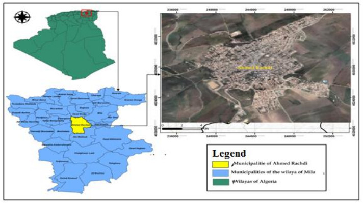
Increasing urbanization related to land pressure and the soil arising from it are aggravating factors of flood risk in urban areas, including storm water runoff. Therefore, urban sanitation networks face an excess of water that exceeds their absorption capacity. This article deals with the effect of impermeability in densely populated urban areas and the function of a combined sewer system under higher rainfall intensities using the Storm Water Management Model (SWMM). The objective is to simulate a possible increase in rainfall intensities for reducing overflow points in the combined sewage system at the study area, which was the city of Ahmed Rachdi, Mila in Algeria. The excessive rainfall intensities were modeled using the SWMM software program to estimate maximum water volumes inside the combined sewage system of the study area. To evaluate the model's performance, a comparison process was used between the values of the flow rates of the pipelines of the sewerage system combined with the design flow rates in the current state and the flow rates of a single modeling of future events available during the study interval. The comparison results showed a good and convergent performance for these models. The results of the flooding volumes using different values of rainfall intensities and different return periods, which were 2, 5, 10 and 25 years, in the modeling of the combined sewage system are 3626, 6888, 8636 and 12676m3, respectively. The suggested scenario included increasing diameters of some pipes in the combined sewage system pipelines. The results using this scenario showed reductions in the total percentage of overflow points from the integrated sewage system of 52.42%, 40.63%, 31.83% and 20.51% using the rainfall intensities for the return periods of 2, 5, 10 and 25 years, respectively. The present study can provide technical support for using software in the planning, controlling and tests of the sewer systems, which contribute to solving the sewer systems' problems.

| [1] | Metcalf, Eddy, Inc. (1981) Wastewater engineering: collection and pumping of waste water, Tchobanoglous, G., Ed. New York: McGraw-Hill Book Company. |
| [2] |
Burian S, Edwards F (2002) Historical Perspectives of Urban Drainage. In Global Solutions for Urban Drainage 2002: 1-16. https://doi.org/10.1061/40644(2002)284 doi: 10.1061/40644(2002)284

|
| [3] | Hussein A, Obaid S, Shahid KN, et al. (2014) Modeling sewerage overflow in an urban residential area using storm water management model. MalaysianJournal of Civil Engineering 26: 163-171. |
| [4] | Safavi HR (2014) Engineering hydrology, 4thedn. Isfahan University of Technology. |
| [5] |
Hassan WH, Nile BK, Al-Masody BA (2017) Climate change effect on storm drainage networks by stormwater management model. Environmental Engineering Research 22: 393-400. https://doi.org/10.4491/eer.2017.036 doi: 10.4491/eer.2017.036
|
| [6] |
Fasheng M, Yiping W, Török Á, et al. (2022) Centrifugal model test on a riverine landslide in the Three Gorges Reservoir induced by rainfall and water level fluctuation.Geoscience Frontiers 13: 101378. https://doi.org/10.1016/j.gsf.2022.101378 doi: 10.1016/j.gsf.2022.101378
|
| [7] |
Miao F, Wu Y, Xie Y, et al. (2018) Prediction of landslide displacement with steplike behavior based on multialgorithm optimization and a support vector regression model. Landslides 15: 475-488. https://doi.org/10.1007/s10346-017-0883-y doi: 10.1007/s10346-017-0883-y
|
| [8] |
Rosburg TT, Nelson PA, Bledsoe BP (2017) Effects of urbanization on flow duration and stream flashiness: a case study of Puget Sound streams, western Washington, USA. JAWRA Journal of the American Water Resources Association 53: 493-507. https://doi.org/10.1111/1752-1688.12511 doi: 10.1111/1752-1688.12511
|
| [9] |
Salerno F, Gaetano V, Gianni T (2018) Urbanization and climate change impacts on surface water quality: Enhancing the resilience by reducing impervious surfaces. Water research 144: 491-502. https://doi.org/10.1016/j.watres.2018.07.058 doi: 10.1016/j.watres.2018.07.058
|
| [10] |
Chang NB, Lu JW, Chui TFM, et al. (2018) Global policy analysis of low impact development for stormwater management in urban regions. Land Use Policy 70: 368-383. https://doi.org/10.1016/j.landusepol.2017.11.024 doi: 10.1016/j.landusepol.2017.11.024
|
| [11] |
Rangari VA, Sridhar V, Umamahesh NV, et al. (2019) Floodplain mapping and management of urban catchment using HEC-RAS: a case study of Hyderabad city. Journal of The Institution of Engineers (India): Series A 100: 49-63. https://doi.org/10.1007/s40030-018-0345-0 doi: 10.1007/s40030-018-0345-0
|
| [12] | Ho G (2000) International Source Book on Environmentally Sound Technologies. Forwastewater and stormwater management. UNEP Division of Technology, Industry and Economics. International Environmental Technology Centre, Osaka/Shiga, 151. |
| [13] |
Jia H, Yao H, Shaw LY (2013) Advances in LID BMPs research and practice for urban runoff control in China. Frontiers of Environmental Science & Engineering 7: 709-720. https://doi.org/10.1007/s11783-013-0557-5 doi: 10.1007/s11783-013-0557-5
|
| [14] |
Barredo JI (2007) Major flood disasters in Europe: 1950-2005. Natural Hazards 42: 125-148. https://doi.org/10.1007/s11069-006-9065-2 doi: 10.1007/s11069-006-9065-2
|
| [15] | National Water Resources Agency (2003) Synthesis study on surface water resources in northern Algeria (Study report), Algeria: Algiers, 36. |
| [16] | National Sanitation Office unit of Mila (1993) Report of Directories wastewater network. |
| [17] |
Yang Y, Sun L, Li R, et al. (2020) Linking a stormwater management model to a novel two-dimensional model for urban pluvial flood modelling. International Journal of Disaster Risk Science 11: 508-518. https://doi.org/10.1007/s13753-020-00278-7 doi: 10.1007/s13753-020-00278-7
|
| [18] |
Adeniyi AG, Michael OD, Assela P (2016) Coupled 1D-2D hydrodynamic inundation model for sewer overflow: Influence of modeling parameters. Water Science 29: 146-155. https://doi.org/10.1016/j.wsj.2015.12.001 doi: 10.1016/j.wsj.2015.12.001
|
| [19] | Mila Water Resources Directorate (2009) Report of Directories |
| [20] | Directorate of urban planning, architecture and construction, wilaya of Mila (2022). |
| [21] | Rossman LA (2010) Stormwater management model user's manual, version 5.0 (p. 276). Cincinnati: National Risk Management Research Laboratory, Office of Research and Development, US Environmental Protection Agency. |
| [22] | Lockie T (2009) Catchment modelling using SWMM. In Modelling Stream at the 49th Water New Zealand Annual Conference and Expo. |
| [23] | Choi NJ (2016) Understanding sewer infiltration and inflow using impulse response functions derived from physics-based models (Doctoral dissertation, the University of Illinois at Urbana-Champaign). |
| [24] | MNSO (National Sanitation Office unit of Mila), (2017). Report of Directories wastewater network. |
| [25] | Steel EW, McGhee TJ (1979) Water Supply and. Sewerage. (McCraw). |
| [26] | Housing statistics (2020) report Communal People's Assembly of the city of Ahmed Rachdi. |
| [27] | World Health Organization (2011) Guidance on water supply and sanitation in extreme weather events, World Health Organization, Regional Office for Europe. |
| [28] | Algerian National Meteorological Office.(ANMO).(2021).Bultin meteorologic |
| [29] |
Rawls WJ, Brakensiek DL, Miller N (1983) Green-Ampt infiltration parameters from soils data. Journal of hydraulic engineering 9: 62-70. https://doi.org/10.1061/(ASCE)0733-9429(1983)109:1(62) doi: 10.1061/(ASCE)0733-9429(1983)109:1(62)
|
| [30] | Richard H (1989) Hydrologic Analyses and Design Englewood Cliffs, New Jersey, 9-10. |
| [31] |
Zaini N, Malek MA, Yusoff M (2015)Application of computational intelligence methods in modeling river flow prediction: A review. In 2015International Conference on Computer, Communications, and Control Technology (I4CT) 2015: 370-374. https://doi.org/10.1109/I4CT.2015.7219600 doi: 10.1109/I4CT.2015.7219600
|
| [32] |
Badieizadeh S, Bahrehmand A, Ahmad DA (2016) Calibration and Evaluation of the HydrologicHydraulic Model SWMM to Simulate Runoff (Case study: Gorgan). Journal of Watershed Management Research 2016: 1-10. https://doi.org/10.29252/jwmr.7.14.10 doi: 10.29252/jwmr.7.14.10
|
| [33] | Kourtis IM, Kopsiaftis G, Bellos V, et al. (2017) Calibration and validation of SWMM model in two urban catchments in Athens, Greece. In International Conference on Environmental Science and Technology (CEST). |
| [34] | Taatpour F, Kouhanestani ZK, Armin M (2019) Evaluating the Performance of Collection and Disposal of Surface Runoff Network Using SWMM Model (Case Study: the City of Likak, Kohgiluyeh and Boyer Ahmad Province). Irrigation Sciences and Engineering 42: 33-48. |
| [35] |
Hendrawan AP (2020) Alternatives of flood control for the Line river, city of Toboali (a case study of the Rawabangun region). In IOP Conference Series: Earth and Environmental Science 437: 012047. https://doi.org/10.1088/1755-1315/437/1/012047 doi: 10.1088/1755-1315/437/1/012047
|
| [36] |
Nile BK (2018) Effectiveness of hydraulic and hydrologic parameters in assessing storm system flooding. Advances in Civil Engineering, 2018. https://doi.org/10.1155/2018/4639172 doi: 10.1155/2018/4639172
|
| [37] | Nile BK, Hassan WH, Alshama GA (2019) Analysis of the effect of climate change on rainfall intensity and expected flooding by using ANN and SWMM programs. ARPN Journal of Engineering and Applied Sciences 14: 974-984. |
| [38] | Li YW, You XY, Ji M, et al. (2010) Optimization of rainwater drainage system based on SWMM model. China Water & Wastewater 26: 40-43. |


Figures(12) / Tables(7)

RAHMOUN Ibrahim, BENMAMAR Saâdia, RABEHI Mohamed. Comparison between different Intensities of Rainfall to identify overflow points in a combined sewer system using Storm Water Management Model[J]. AIMS Environmental Science, 2022, 9(5): 573-592. doi: 10.3934/environsci.2022034


 DownLoad: