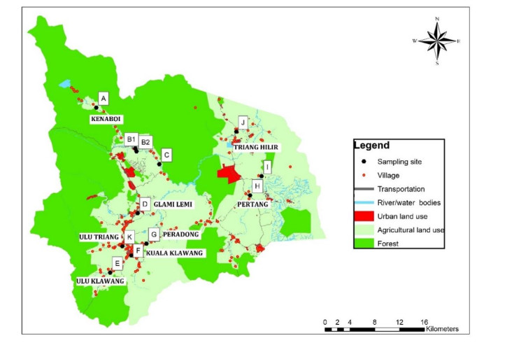
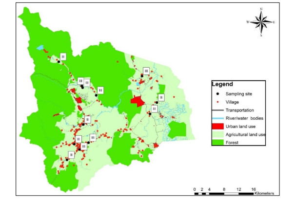
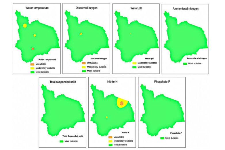
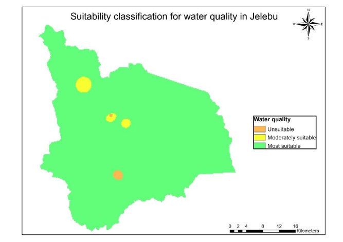
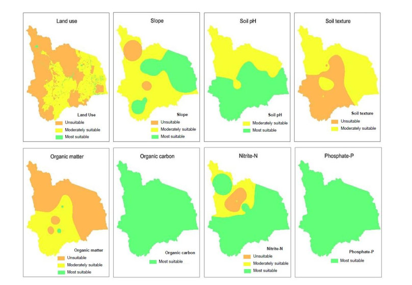
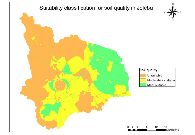
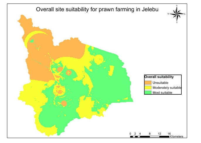
Water and soil qualities play significant roles in the farming of giant freshwater prawn. The study evaluated water and soil qualities for giant freshwater prawn farming site suitability by using Analytic Hierarchy Process (AHP) and Geographic Information System (GIS) in Jelebu, Malaysia. The water quality parameters measured were biochemical oxygen demand, chemical oxygen demand, ammonia nitrogen, pH, dissolved oxygen, water temperature, total suspended solids, nitrite concentration and phosphate concentration, meanwhile soil qualities investigated were land use, slope, pH, texture, organic carbon and organic matter. Site suitability analysis can assist to identify the best location for prawn production. Specialist's opinions were used to rank the level of preference and significance of each of the parameter while the pairwise comparison matrix was applied to calculate the weight of each parameter for prawn farming. There are about 45.41% of the land was most suitable, 28.89% was moderately suitable while 25.69% was found unsuitable for prawn farming. The combination of AHP and GIS could give a better database and guide map for planners and decision-makers to take more rewarding decisions when apportioning the land for prawn farming, for better productivity.
Citation: Rosazlin Abdullah, Firuza Begham Mustafa, Subha Bhassu, Nur Aziaty Amirah Azhar, Benjamin Ezekiel Bwadi, Nur Syabeera Begum Nasir Ahmad, Aaronn Avit Ajeng. Evaluation of water and soil qualities for giant freshwater prawn farming site suitability by using the AHP and GIS approaches in Jelebu, Negeri Sembilan, Malaysia[J]. AIMS Geosciences, 2021, 7(3): 507-528. doi: 10.3934/geosci.2021029
Water and soil qualities play significant roles in the farming of giant freshwater prawn. The study evaluated water and soil qualities for giant freshwater prawn farming site suitability by using Analytic Hierarchy Process (AHP) and Geographic Information System (GIS) in Jelebu, Malaysia. The water quality parameters measured were biochemical oxygen demand, chemical oxygen demand, ammonia nitrogen, pH, dissolved oxygen, water temperature, total suspended solids, nitrite concentration and phosphate concentration, meanwhile soil qualities investigated were land use, slope, pH, texture, organic carbon and organic matter. Site suitability analysis can assist to identify the best location for prawn production. Specialist's opinions were used to rank the level of preference and significance of each of the parameter while the pairwise comparison matrix was applied to calculate the weight of each parameter for prawn farming. There are about 45.41% of the land was most suitable, 28.89% was moderately suitable while 25.69% was found unsuitable for prawn farming. The combination of AHP and GIS could give a better database and guide map for planners and decision-makers to take more rewarding decisions when apportioning the land for prawn farming, for better productivity.

| [1] |
Hossain MS, Das NG (2010) GIS-based multi-criteria evaluation to land suitability modelling for giant prawn (Macrobrachium rosenbergii) farming in Companigonj Upazila of Noakhali, Bangladesh. Comput Electron Agric 70: 172-186. doi: 10.1016/j.compag.2009.10.003

|
| [2] | Ezekiel BB, Firuza B, Mohammad L, et al. (2018) Analysis of Factors for Determining Suitable Site for Giant Freshwater Prawn (Macrobrachium rosenbergii) Farming Through the Local Knowledge in Negeri Sembilan of Peninsular Malaysia. Pertanika J Soc Sci Humanit 26: 2867-2882. |
| [3] |
Zafar M, Haque M, Aziz M, et al. (2015) Study on water and soil quality parameters of shrimp and prawn farming in the southwest region of Bangladesh. J Bangladesh Agric Univ 13: 153-160. doi: 10.3329/jbau.v13i1.28732
|
| [4] | Food and Agriculture Organization, Aquaculture, 2020. Available from: http://www.fao.org/fishery/en. |
| [5] |
Banu R, Christianus A (2016) Giant freshwater prawn Macrobrachium rosenbergii farming: A review on its current status and prospective in Malaysia. J Aquacul Res Dev 7: 1-5. doi: 10.4172/2155-9546.1000423
|
| [6] | New MB, Valenti WC, Tidwell JH, et al. (2009) Freshwater prawns: biology and farming. John Wiley & Sons. |
| [7] | Islam MM, Ahmed MK, Shahid MA, et al. (2009) Determination of land cover changes and suitable shrimp farming area using remote sensing and GIS in Southwestern Bangladesh. Int J Ecol Dev 12: 28-41. |
| [8] |
Mustafa FB, Bwadi BE (2018) Determination of Optimal Freshwater Prawn Farming Site Locations using GIS and Multicriteria Evaluation. J Coastal Res 82: 41-54. doi: 10.2112/SI82-006.1
|
| [9] |
Joerin F, Thériault M, Musy A (2001) Using GIS and outranking multicriteria analysis for land-use suitability assessment. Int J Geogr Inf Sci 15: 153-174. doi: 10.1080/13658810051030487
|
| [10] |
Sanchez-Jerez P, Karakassis I, Massa F, et al. (2016) Aquaculture's struggle for space: the need for coastal spatial planning and the potential benefits of Allocated Zones for Aquaculture (AZAs) to avoid conflict and promote sustainability. Aquacult Environ Interact 8: 41-54. doi: 10.3354/aei00161
|
| [11] |
Höhn J, Lehtonen E, Rasi S, et al. (2014) A Geographical Information System (GIS) based methodology for determination of potential biomasses and sites for biogas plants in southern Finland. Appl Energy 113: 1-10. doi: 10.1016/j.apenergy.2013.07.005
|
| [12] | Sánchez-Moreno JF, Farshad A, Pilesjö P (2013) Farmer or expert; a comparison between three land suitability assessments for upland Rice and rubber in Phonexay District, Lao Pdr. Ecopersia 1: 235-260. |
| [13] |
Baja S, Chapman DM, Dragovich D (2007) Spatial based compromise programming for multiple criteria decision making in land use planning. Environ Model Assess 12: 171-184. doi: 10.1007/s10666-006-9059-1
|
| [14] | Singha C, Swain KC (2016) Land suitability evaluation criteria for agricultural crop selection: A review. Agric Rev 37. |
| [15] |
Akıncı H, Özalp AY, Turgut B (2013) Agricultural land use suitability analysis using GIS and AHP technique. Comput Electron Agric 97: 71-82. doi: 10.1016/j.compag.2013.07.006
|
| [16] |
Farkan M, Setiyanto D, Widjaja R (2017) Assessment area development of sustainable shrimp culture ponds (case ctudy the gulf coast Banten). IOP Conf Ser Earth Environ Sci 54: 012077. doi: 10.1088/1755-1315/54/1/012077
|
| [17] | Setiawan Y, Pertiwi DGBCS (2014) Evaluation of Land Suitability for Brackishwatershrimp Farming using GIS in Mahakam Delta, Indonesia. Evaluation 4. |
| [18] |
Ullah KM, Mansourian A (2016) Evaluation of Land Suitability for Urban Land—Use Planning: Case Study D haka City. Trans GIS 20: 20-37. doi: 10.1111/tgis.12137
|
| [19] | Zarkesh MK, Ghoddusi J, Zaredar N, et al. (2010) Application of spatial analytical hierarchy process model in land use planning. J Food Agric Environ 8: 970-975. |
| [20] | Kumar V, Jain K (2017) Site suitability evaluation for urban development using remote sensing, GIS and analytic hierarchy process (AHP), Proceedings of International Conference on Computer Vision and Image Processing, Springer, 377-388. |
| [21] | Salui CL, Hazra PB (2017) Geospatial Analysis for Industrial Site Suitability Using AHP Modeling: A Case Study, Environment and Earth Observation, Springer, 3-21. |
| [22] |
Hossain MS, Chowdhury SR, Das NG, et al. (2009) Integration of GIS and multicriteria decision analysis for urban aquaculture development in Bangladesh. Landscape Urban Plann 90: 119-133. doi: 10.1016/j.landurbplan.2008.10.020
|
| [23] |
Morckel VC (2017) Using suitability analysis to prioritize demolitions in a legacy city. Urban Geogr 38: 90-111. doi: 10.1080/02723638.2016.1147756
|
| [24] |
Chandio IA, Matori A, Yusof K, et al. (2014) GIS-basedland suitability analysis of sustainable hillside development. Procedia Eng 77: 87-94. doi: 10.1016/j.proeng.2014.07.009
|
| [25] | Trinh T, Wu D, Huang J, et al. (2016) Application of the analytical hierarchy process (AHP) for landslide susceptibility mapping: A case study in Yen Bai province, Viet Nam, CRC Press, 275. |
| [26] |
Rahmat ZG, Niri MV, Alavi N, et al. (2017) Landfill site selection using GIS and AHP: a case study: Behbahan, Iran. KSCE J Civ Eng 21: 111-118. doi: 10.1007/s12205-016-0296-9
|
| [27] |
Şener Ş, Şener E, Nas B, et al. (2010) Combining AHP with GIS for landfill site selection: a case study in the Lake Beyşehir catchment area (Konya, Turkey). Waste Manage 30: 2037-2046. doi: 10.1016/j.wasman.2010.05.024
|
| [28] | Malczewski J, Rinner C (2015) GIScience, Spatial Analysis, and Decision Support, Multicriteria Decision Analysis in Geographic Information Science, Springer, 3-21. |
| [29] |
Goodridge W, Bernard M, Jordan R, et al. (2017) Intelligent diagnosis of diseases in plants using a hybrid Multi-Criteria decision making technique. Comput Electron Agric 133: 80-87. doi: 10.1016/j.compag.2016.12.003
|
| [30] | Abu-Taha R (2011) Multi-criteria applications in renewable energy analysis: A literature review, IEEE, 1-8. |
| [31] | Mendoza GA (2000) GIS-based multicriteria approaches to land use suitability assessment and allocation. United States Department of Agriculture Forest Service General Technical Report NC, 89-94. |
| [32] |
Dehe B, Bamford D (2015) Development, test and comparison of two Multiple Criteria Decision Analysis (MCDA) models: A case of healthcare infrastructure location. Expert Syst Appl 42: 6717-6727. doi: 10.1016/j.eswa.2015.04.059
|
| [33] |
Dhami I, Deng J, Strager M, et al. (2017) Suitability-sensitivity analysis of nature-based tourism using geographic information systems and analytic hierarchy process. J Ecotourism 16: 41-68. doi: 10.1080/14724049.2016.1193186
|
| [34] |
Bwadi BE, Mustafa FB, Ali ML, et al. (2019) Spatial analysis of water quality and its suitability in farming giant freshwater prawn (Macrobrachium rosenbergii) in Negeri Sembilan region, Peninsular Malaysia. Singapore J Trop Geogr 40: 71-91. doi: 10.1111/sjtg.12250
|
| [35] | Department of Fisheries Laporan Tahunan Dan Penyata Kewangan LKIM Tahun 2014. Available from: https://www.lkim.gov.my/wp-content/uploads/2015/10/1.-FINAL-LAPORAN-TAHUNAN-2014.pdf |
| [36] |
Naubi I, Zardari NH, Shirazi SM, et al. (2016) Effectiveness of Water Quality Index for Monitoring Malaysian River Water Quality. Pol J Environ Stud 25: 231-239. doi: 10.15244/pjoes/60109
|
| [37] | National Water Quality Standards For Malaysia. Available from: https://www.doe.gov.my/portalv1/wp-content/uploads/2019/05/Standard-Kualiti-Air-Kebangsaan.pdf. |
| [38] | Wastewater Sampling Method, 2013. Available from: http://www.aquaculture.asia/files/PMNQ%20WQ%20standard%202.pdf. |
| [39] | Standard Methods for the Examination of Water and Wastewater 23rd edition (APHA, AWWA, WEF), 2017. Available from: https://www.wef.org/resources/publications/books/StandardMethods/. |
| [40] |
Thunjai T, Boyd CE, Dube K (2001) Poind soil pH measurement. J World Aquacul Soc 32: 141-152. doi: 10.1111/j.1749-7345.2001.tb00365.x
|
| [41] | Chaikaew P, Chavanich S (2017) Spatial variability and relationship of mangrove soil organic matter to organic carbon. Appl Environ Soil Sci 2017. |
| [42] | Saia S, Salvucci T, Zhang W (2018) Ion Chromatography Procedure. Available from: http://soilandwater.bee.cornell.edu/tools/equipment/IC_Protocol.pdf. |
| [43] | Water Quality Criteria and Standards for Freshwater and Marine Aquaculture. Available from: http://aquaculture.asia/files/PMNQ%20WQ%20standard%202.pdf. |
| [44] |
Hadipour A, Vafaie F, Hadipour V (2015) Land suitability evaluation for brackish water aquaculture development in coastal area of Hormozgan, Iran. Aquacult Int 23: 329-343. doi: 10.1007/s10499-014-9818-y
|
| [45] |
New MB, Nair CM (2012) Global scale of freshwater prawn farming. Aquacult Res 43: 960-969. doi: 10.1111/j.1365-2109.2011.03008.x
|
| [46] | Food and Agriculture Organization, Farming freshwater prawns—A manual for the culture of the giant river prawn (Macrobrachium rosenbergii). 2020. Available from: http://www.fao.org/3/y4100e/y4100e00.htm. |
| [47] |
Mallasen M, Valenti WC (2005) Larval development of the giant river prawn Macrobrachium rosenbergii at different ammonia concentrations and pH values. J World Aquacul Soc 36: 32-41. doi: 10.1111/j.1749-7345.2005.tb00128.x
|
| [48] | Food and Agriculture Organization of the United Nations, A framework for land evaluation. 1976. Available from: https://edepot.wur.nl/149437. |
| [49] |
Rossiter DG (1996) A theoretical framework for land evaluation. Geoderma 72: 165-190. doi: 10.1016/0016-7061(96)00031-6
|
| [50] | New MB, Kutty MN (2010) Commercial freshwater prawn farming and enhancement around the world. Freshwater Prawns; Biology and Farming, 346-399. |
| [51] |
Nguyen TT, Verdoodt A, Van Y T, et al. (2015) Design of a GIS and multi-criteria based land evaluation procedure for sustainable land-use planning at the regional level. Agric Ecosyst Environ 200: 1-11. doi: 10.1016/j.agee.2014.10.015
|
| [52] | Capraz O, Meran C, Wörner W, et al. (2015) Using AHP and TOPSIS to evaluate welding processes for manufacturing plain carbon stainless steel storage tank. Arch Mater Sci 76: 157-162. |
| [53] |
García JL, Alvarado A, Blanco J, et al. (2014) Multi-attribute evaluation and selection of sites for agricultural product warehouses based on an analytic hierarchy process. Comput Electron Agric 100: 60-69. doi: 10.1016/j.compag.2013.10.009
|
| [54] |
Saaty TL (2004) Decision making—the analytic hierarchy and network processes (AHP/ANP). J Syst Sci Syst Eng 13: 1-35. doi: 10.1007/s11518-006-0151-5
|
| [55] |
Pramanik MK (2016) Site suitability analysis for agricultural land use of Darjeeling district using AHP and GIS techniques. Model Earth Sys Environ 2: 56. doi: 10.1007/s40808-016-0116-8
|
| [56] |
Park S, Jeon S, Kim S, et al. (2011) Prediction and comparison of urban growth by land suitability index mapping using GIS and RS in South Korea. Landscape Urban Plann 99: 104-114. doi: 10.1016/j.landurbplan.2010.09.001
|
| [57] | Öztürk D, Batuk F (2010) Konumsal karar problemlerinde analitik hiyerarşi yönteminin kullanılması. Sigma Mühendislik ve Fen Bilimleri Derg 28: 124-137. |
| [58] | Apak S, Orbak I, Tombus A, et al. (2015) Analyzing logistics firms business performance. Sci Bull Mircea Cel Batran Naval Acad 18: 180. |
| [59] | Malczewski J (1999) GIS and multicriteria decision analysis, John Wiley & Sons. |
| [60] | Huang YF, Ang SY, Lee KM, et al. (2015) Quality of water resources in Malaysia. Res Pract Water Qual 3: 65-94. |
| [61] |
Ferreira N, Bonetti C, Seiffert W (2011) Hydrological and water quality indices as management tools in marine shrimp culture. Aquaculture 318: 425-433. doi: 10.1016/j.aquaculture.2011.05.045
|
| [62] |
Cheng W, Chen JC (2000) Effects of pH, temperature and salinity on immune parameters of the freshwater prawn Macrobrachium rosenbergii. Fish Shellfish Immunol 10: 387-391. doi: 10.1006/fsim.2000.0264
|
| [63] | Boyd CE (2017) General relationship between water quality and aquaculture performance in ponds, Fish Dis 147-166. |
| [64] | Hai NT, Lili Y, Qigen L, et al. (2015) Assessment of water quality of giant freshwater prawn (Macrobrachium rosenbergii) in culture ponds in Zhejiang of China. Int J Fish Aquat Stud 2: 45-55. |
| [65] | Osmi SAC, Ishak WFW, Azman MA, et al. (2018) Recent assessment of physico-chemical water quality in Malacca River using water quality index and statistical analysis, IOP Conf Ser Earth Environ Sci 169: 012071. |
| [66] | Khoda Bakhsh H, Chopin T (2011) Water quality and nutrient aspects in recirculating aquaponic production of the freshwater prawn, Macrobrachium rosenbergii and the lettuce, Lactuca sativa. Available from: http://hdl.handle.net/10919/90643. |
| [67] | Alam T (2015) Estimation of Chemical Oxygen Demand in WasteWater using UV-VIS Spectroscopy. Available from: https://core.ac.uk/download/pdf/56379601.pdf. |
| [68] | Boyd CE, Wood C, Thunjai T (2002) Aquaculture pond bottom soil quality management, Pond Dynamics/Aquaculture Collaborative Research Support Program. Oregon. |
| [69] |
Gardi C, Visioli G, Conti FD, et al. (2016) High nature value farmland: assessment of soil organic carbon in Europe. Front Environ Sci 4: 47. doi: 10.3389/fenvs.2016.00047
|
Figures(7) / Tables(9)

Rosazlin Abdullah, Firuza Begham Mustafa, Subha Bhassu, Nur Aziaty Amirah Azhar, Benjamin Ezekiel Bwadi, Nur Syabeera Begum Nasir Ahmad, Aaronn Avit Ajeng. Evaluation of water and soil qualities for giant freshwater prawn farming site suitability by using the AHP and GIS approaches in Jelebu, Negeri Sembilan, Malaysia[J]. AIMS Geosciences, 2021, 7(3): 507-528. doi: 10.3934/geosci.2021029


 DownLoad: