The ups and downs of stock indexes are one of the most concerned issues for investors in the stock market. To improve the accuracy of stock index prediction, this paper compares traditional K-Fold Cross-Validation (KCV) and three cross-validation methods in the Radial Basis Function Support Vector Regression (RBF-SVR) model. They are named as Abandon Tail Cross-Validation (ATCV), Sequential Division Cross-Validation (SCV) and Gap Sequential Division Cross-Validation (GSCV). It is found that KCV has very limited validation ability for stock indexes time series data with no certain relevance. However, SCV and GSCV with small gap perform better, with high accuracy about 88% and small error about 2%. This research shows that the establishment of time series forecasting models for stock indexes needs to pay more attention to cross-validation methods, which cannot randomly dividing training set and test set. It is strongly recommended to use SCV and GSCV instead of KCV. In addition, the choice of the penalty parameter C and the radial basis kernel function parameter γ largely determines the accuracy and reliability of RBF-SVR stock index prediction model.
Citation: Feite Zhou. Cross-validation research based on RBF-SVR model for stock index prediction[J]. Data Science in Finance and Economics, 2021, 1(1): 1-20. doi: 10.3934/DSFE.2021001
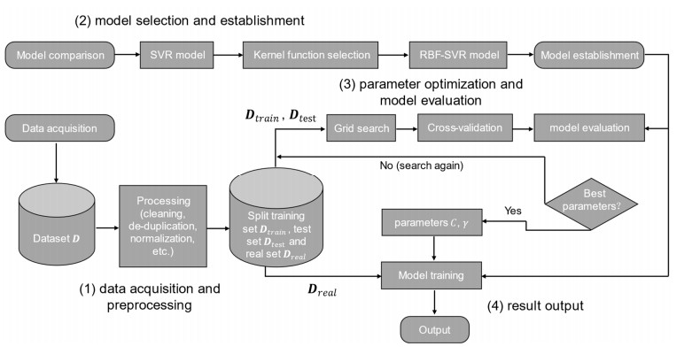
The ups and downs of stock indexes are one of the most concerned issues for investors in the stock market. To improve the accuracy of stock index prediction, this paper compares traditional K-Fold Cross-Validation (KCV) and three cross-validation methods in the Radial Basis Function Support Vector Regression (RBF-SVR) model. They are named as Abandon Tail Cross-Validation (ATCV), Sequential Division Cross-Validation (SCV) and Gap Sequential Division Cross-Validation (GSCV). It is found that KCV has very limited validation ability for stock indexes time series data with no certain relevance. However, SCV and GSCV with small gap perform better, with high accuracy about 88% and small error about 2%. This research shows that the establishment of time series forecasting models for stock indexes needs to pay more attention to cross-validation methods, which cannot randomly dividing training set and test set. It is strongly recommended to use SCV and GSCV instead of KCV. In addition, the choice of the penalty parameter C and the radial basis kernel function parameter γ largely determines the accuracy and reliability of RBF-SVR stock index prediction model.

| [1] | Achkar R, Elias-Sleiman F, Ezzidine H, et al. (2018) Comparison of BPA-MLP and LSTM-RNN for stocks prediction. 2018 6th International Symposium on Computational and Business Intelligence (ISCBI). 2018: 48-51. |
| [2] | Adebiyi AA, Adewumi AO, Ayo CK (2014) Stock price prediction using the ARIMA model. 2014 UKSim-AMSS 16th International Conference on Computer Modelling and Simulation. 2014: 106-112. |
| [3] |
Bergmeir C, Benítez JM (2012) On the use of cross-validation for time series predictor evaluation. Inform Sci 191: 192-213. doi: 10.1016/j.ins.2011.12.028

|
| [4] |
Bergmeir C, Hyndman RJ, Koo B (2018) A note on the validity of cross-validation for evaluating autoregressive time series prediction. Comput Stats Data Anal 120: 70-83. doi: 10.1016/j.csda.2017.11.003
|
| [5] | Cawley GC (2006) Leave-one-out cross-validation based model selection criteria for weighted LS-SVMs. The 2006 IEEE International Joint Conference on Neural Network Proceedings. 2006: 1661-1668. |
| [6] |
Choudhury S, Ghosh S, Bhattacharya A, et al. (2014) A real time clustering and SVM based price-volatility prediction for optimal trading strategy. Neurocomputing 131: 419-426. doi: 10.1016/j.neucom.2013.10.002
|
| [7] | Cortes C, Vapnik V (1995) Support-vector networks. Mach Learn 20: 273-297. |
| [8] | Devi KN, Bhaskaran VM, Kumar GP (2015) Cuckoo optimized SVM for stock market prediction. 2015 International Conference on Innovations in Information, Embedded and Communication Systems (ICIIECS). 2015: 1-5. |
| [9] | Han SJ, Cao QB, Han M (2012) Parameter selection in SVM with RBF kernel function. World Automation Congress 2012. 2012: 1-4. |
| [10] |
Heo JY, Yang JY (2016) Stock price prediction based on financial statements using SVM. Int J Hybri Inform Technol 9: 57-66. doi: 10.14257/ijhit.2016.9.2.05
|
| [11] | Hjort UH (1982) Model selection and forward validation. Scand J Stat 9: 95-105. |
| [12] |
Hochreiter S, Schmidhuber J (1997) Long short-term memory. Neural Comput 9: 1735-1780. doi: 10.1162/neco.1997.9.8.1735
|
| [13] |
Huang CL, Dun JF (2008) A distributed PSO-SVM hybrid system with feature selection and parameter optimization. Appl Soft Comput 8: 1381-1391. doi: 10.1016/j.asoc.2007.10.007
|
| [14] |
Huang W, Nakamori Y, Wang SY (2004) Forecasting stock market movement direction with support vector machine. Comput Oper Res 32: 2513-2522. doi: 10.1016/j.cor.2004.03.016
|
| [15] | Hui X, Wu Y (2012) Research on simple moving average trading system based on SVM. 2012 International Conference on Management Science & Engineering 19th Annual Conference Proceedings. 2012: 1393-1397. |
| [16] | Goodfellow I (2016) Support vector machines, In: Goodfellow I, Bengio Y, Courville A, Deep learning, 2 Eds., The MIT Press, 88-90. |
| [17] | Jarrett JE, Kyper E (2011) ARIMA modeling with intervention to forecast and analyze Chinese stock prices. Int J Eng Bus Manage 3: 53-58. |
| [18] |
Kara Y, Boyacioglu MA, Ömer KB (2011). Predicting direction of stock price index movement using artificial neural networks and support vector machines: the sample of the Istanbul stock exchange. Expert Sys Appl 38: 5311-5319. doi: 10.1016/j.eswa.2010.10.027
|
| [19] |
Karanasos M, Kim J (2003) Moments of the ARMA-EGARCH model. Economet J 6: 146-166. doi: 10.1111/1368-423X.00104
|
| [20] | Karmiani D, Kazi R, Nambisan A, et al. (2019) Comparison of predictive algorithms: backpropagation, SVM, LSTM and Kalman Filter for stock market. 2019 Amity International Conference on Artificial Intelligence (AICAI). 2019: 228-234. |
| [21] |
Lee CM (2009) Using support vector machine with a hybrid feature selection method to the stock trend prediction. Expert Syst Appl 36: 10896-10904. doi: 10.1016/j.eswa.2009.02.038
|
| [22] | Li CH, Lin CT, Kuo BC, et al. (2010) An automatic method for selecting the parameter of the RBF kernel function to support vector machines. 2010 IEEE International Geoscience and Remote Sensing Symposium. 2010: 836-839. |
| [23] | Li ZR, Li CJ, Zhu H (2021) Parameter optimization of HVAC load forecasting model based on Support Vector Regression. Build Energy Effic 49: 43-48. |
| [24] | Lin Y, Guo H, Hu J (2013) An SVM-based approach for stock market trend prediction. 2013 International Joint Conference on Neural Networks (IJCNN). 2013: 1-7. |
| [25] | Liu Y, Du J (2015) Parameter optimization of the SVM for big data. 2015 8th International Symposium on Computational Intelligence and Design (ISCID). 2015: 341-344 |
| [26] |
Makridakis S, Hibon M (2000) The M3-Competition: results, conclusions, and implications. Int J Forecast 16: 451-476. doi: 10.1016/S0169-2070(00)00057-1
|
| [27] |
Marković I, Stojanović M, Stanković J, et al. (2017) Stock market trend prediction using AHP and weighted kernel LS-SVM. Soft Comput 21: 5387-5398. doi: 10.1007/s00500-016-2123-0
|
| [28] | Naeini MP, Taremian H, Hashemi HB (2010) Stock market value prediction using neural networks. 2010 International Conference on Computer Information Systems and Industrial Management Applications (CISIM). 2010: 132-136. |
| [29] | Narayan PK (2006). The behaviour of US stock prices: Evidence from a threshold autoregressive model. Math Comput Simulat 71: 103-108. |
| [30] | Nivetha RY, Dhaya C (2017) Developing a prediction model for stock analysis. 2017 International Conference on Technical Advancements in Computers and Communications (ICTACC). 2017: 1-3. |
| [31] |
Pai PF, Lin CS (2005). A hybrid ARIMA and support vector machines model in stock price forecasting. Omega 33: 497-505. doi: 10.1016/j.omega.2004.07.024
|
| [32] |
Roberts DR, Bahn V, Ciuti S, et al. (2017). Cross-validation strategies for data with temporal, spatial, hierarchical, or phylogenetic structure. Ecography 40: 913-929. doi: 10.1111/ecog.02881
|
| [33] |
Rojas I, Valenzuela O, Rojas F, et al. (2008) Soft-computing techniques and ARMA model for time series prediction. Neurocomputing 71: 519-537. doi: 10.1016/j.neucom.2007.07.018
|
| [34] | Salam MA (2015) Comparative study between FPA, BA, MCS, ABC, and PSO algorithms in training and optimizing of LS-SVM for stock market prediction. Int J Adv Comput Res 5: 35-45. |
| [35] |
Sapankevych NI, Sankar R (2009) Time series prediction using support vector machines. IEEE Comput Intell M 4: 24-38. doi: 10.1109/MCI.2009.932254
|
| [36] | Selvin S, Vinayakumar R, Gopalakrishnan EA, et al. (2017) Stock price prediction using LSTM, RNN and CNN-sliding window model. 2017 International Conference on Advances in Computing, Communications and Informatics (ICACCI). 2017: 1643-1647. |
| [37] | Stone M (1974) Cross-Validatory Choice and Assessment of Statistical Prediction. J Roy Stat Soc 36: 111-147. |
| [38] |
Syarif I, Prugel-Bennett A, Wills G (2016) SVM parameter optimization using grid search and genetic algorithm to improve classification performance. Telkomnika 14: 1502-1509. doi: 10.12928/telkomnika.v14i4.3956
|
| [39] |
Thissen U, Van Brakel R, Weijer AP, et al. (2003) Using support vector machines for time series prediction. Chemometr Intell Lab 69: 35-49. doi: 10.1016/S0169-7439(03)00111-4
|
| [40] | Turchenko V, Beraldi P, Simone FD, et al. (2011) Short-term stock price prediction using MLP in moving simulation mode. The 6th IEEE International Conference on Intelligent Data Acquisition and Advanced Computing Systems. 2011: 666-671. |
| [41] |
Vasyl G, Bastian G, Roman L (2012) The conditional autoregressive Wishart model for multivariate stock market volatility. J Econometrics 167: 211-223. doi: 10.1016/j.jeconom.2011.11.004
|
| [42] |
Wei LY, Cheng CH, Wu HH (2014) A hybrid ANFIS based on n-period moving average model to forecast TAIEX stock. Appl Soft Comput J 19: 86-92. doi: 10.1016/j.asoc.2014.01.022
|
| [43] |
Wen F, Xiao J, Zhifang HE, et al. (2014) Stock price prediction based on SSA and SVM. Procedia Comput Sci 31: 625-631. doi: 10.1016/j.procs.2014.05.309
|
| [44] | Yadav S, Shukla S (2016) Analysis of K-Fold Cross-Validation over hold-out validation on colossal datasets for quality classification. 2016 IEEE 6th International Conference on Advanced Computing (IACC). 2016: 7 8-83. |
| [45] |
Yu HH, Chen RD, Zhang GP (2014) An SVM stock selection model within PCA. Procedia Comput Sci 31: 406-412. doi: 10.1016/j.procs.2014.05.284
|
| [46] | Zhou ZH (2016) Support vector machines, In: Zhou ZH, Machine learning, Chinese version, 2 Eds., Bei Jing: The Tsinghua University Press, 121-145. |
| [47] | Zhu WG, Li YX, Yang WQ, et al. (2021). Short-term load forecast based on K-Fold Cross-Validation and stacking integration. J Electr Pow Sci Technol 36: 87-95. |
 DSFE-01-01-001-s001.csv DSFE-01-01-001-s001.csv |
 |


Figures(7) / Tables(7)
Feite Zhou. Cross-validation research based on RBF-SVR model for stock index prediction[J]. Data Science in Finance and Economics, 2021, 1(1): 1-20. doi: 10.3934/DSFE.2021001


 DownLoad: