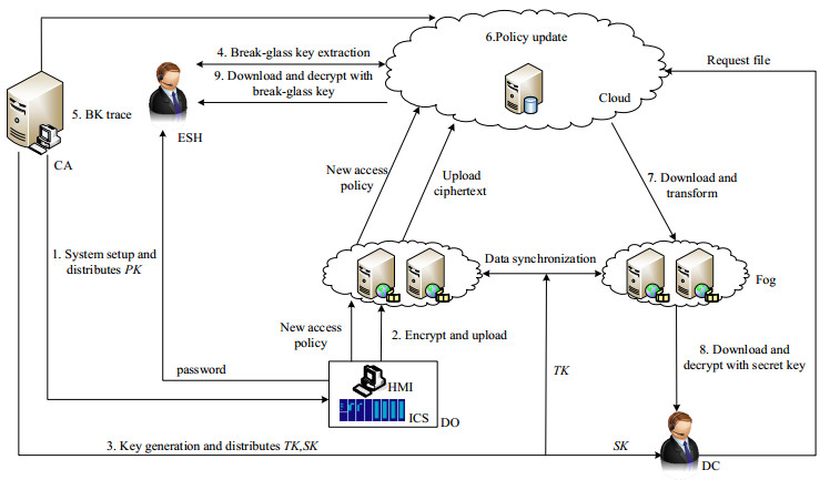
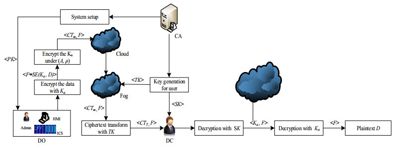
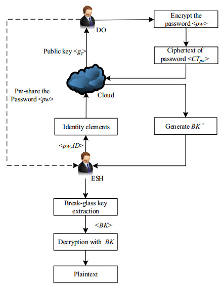
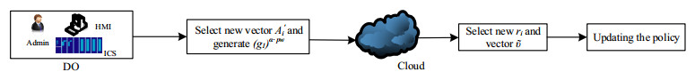
In the era of Industry4.0, cloud-assisted industrial control system (ICS) is considered to be the most promising technology for industrial processing automation systems. However, the emerging attack techniques targeted at ICS underlines the importance of data security. To protect the data from the unauthorized accesses, attribute-based encryption is utilized to meet the requirement of confidentiality and access control demand of an open network environment. In ICS scenarios, it is critically important to offer the timely and efficient service, especially in the emergency situations. This paper proposes an efficient access control strategy that enables two access modes: attribute-based access and emergency break-glass access. Normally, users can access the encrypted data as long as their attributes satisfy the access policy specified by the data owner. In emergency cases, emergency situation handlers can override the access control policy of the encrypted data by the break-glass access capability. To eliminate the overhead for data consumers, the scheme outsources the data decryption and policy updating to the semi-trusted fog and cloud. The scheme also implements the CP-ABE scheme in terms of an asymmetric Type-3 pairings instead of the symmetric Type-1 pairings, which are inefficient and have security issues. Finally, the paper analyses the security of the scheme, evaluates its performance, and compares it with related works.
Citation: Yuanfei Tu, Jing Wang, Geng Yang, Ben Liu. An efficient attribute-based access control system with break-glass capability for cloud-assisted industrial control system[J]. Mathematical Biosciences and Engineering, 2021, 18(4): 3559-3577. doi: 10.3934/mbe.2021179
In the era of Industry4.0, cloud-assisted industrial control system (ICS) is considered to be the most promising technology for industrial processing automation systems. However, the emerging attack techniques targeted at ICS underlines the importance of data security. To protect the data from the unauthorized accesses, attribute-based encryption is utilized to meet the requirement of confidentiality and access control demand of an open network environment. In ICS scenarios, it is critically important to offer the timely and efficient service, especially in the emergency situations. This paper proposes an efficient access control strategy that enables two access modes: attribute-based access and emergency break-glass access. Normally, users can access the encrypted data as long as their attributes satisfy the access policy specified by the data owner. In emergency cases, emergency situation handlers can override the access control policy of the encrypted data by the break-glass access capability. To eliminate the overhead for data consumers, the scheme outsources the data decryption and policy updating to the semi-trusted fog and cloud. The scheme also implements the CP-ABE scheme in terms of an asymmetric Type-3 pairings instead of the symmetric Type-1 pairings, which are inefficient and have security issues. Finally, the paper analyses the security of the scheme, evaluates its performance, and compares it with related works.

| [1] |
A. Sajid, H. Abbas, K. Saleem, Cloud-assisted Iot-based SCADA systems security: a review of the state of the art and furture challenges, IEEE Access, 4 (2016), 1375-1384. doi: 10.1109/ACCESS.2016.2549047

|
| [2] | T. Ma, H. Rong, Y. Hao, J. Cao, Y. Tian, M. A. Al-Rodhaan, A novel sentiment polarity detection framework for Chinese, IEEE Trans. Affective Comput., (2019), forthcoming. |
| [3] |
H. Rong, T. Ma, J. Cao, Y. Tian, A. Al-Dhelaan, M. Al-Rodhaan, Deep rolling: a novel emotion prediction model for a multi-participant communication context, Inf. Sci., 488 (2019), 158-180. doi: 10.1016/j.ins.2019.03.023
|
| [4] |
A. Ouaddaha, H. Mousannif, A. A. Elkalam, A. A. Ouahman, Access control in the Internet of Things: big challenges and new opportunities, Comput. Networks, 112 (2017), 237-262. doi: 10.1016/j.comnet.2016.11.007
|
| [5] |
S. Plaga, N. Wiedermann, S. D. Anton, S. Tatschner, H. Schotten, T. Newe, Securing future decentralised industrial IoT infrastructures: challenges and free open source solutions, Future Gener. Comput. Syst., 93 (2019), 596-608. doi: 10.1016/j.future.2018.11.008
|
| [6] | B. Al-Otibi, N. Al-Nabhan, Y. Tian, Privacy-preserving vehicular rogue node detection scheme for fog computing, Sensors, 19 (2019), 965. |
| [7] |
Y. Tian, M. M. Kaleemullah, M. A. Rodhaan, B. Song, A. Al-Dhelaan, T. Ma, A privacy preserving location service for Cloud-of-Things system, J. Parallel Distrib. Comput., 123 (2019), 215-222. doi: 10.1016/j.jpdc.2018.09.005
|
| [8] |
B. Song, M. M. Hassan, A. Alamri, A. Alelaiwi, Y. Tian, M. Pathan, A. Almogren, A two-stage approach for task and resource management in multimedia cloud environment, Computing, 98 (2016), 119-145. doi: 10.1007/s00607-014-0411-z
|
| [9] | A. Shahzad, S. Musa, A. Aborujilah, M. Irfan, Industrial Control Systems (ICSs) vulnerabilities analysis and SCADA security enhancement using testbed encryption, in Proceedings of the 8th International Conference on Ubiquitous Information Management and Communication, ACM, 2014. |
| [10] |
A. Rahman, E. Hassanain, M. Hossain, Towards a secure mobile edge computing framework for Hajj, IEEE Access, 5 (2017), 11768-11781. doi: 10.1109/ACCESS.2017.2716782
|
| [11] |
W. Teng, G. Yang, Y. Xiang, T. Zhang, D. Wang, Attribute-based access control with constant-size ciphertext in cloud computing, IEEE Trans. Cloud Comput., 5 (2017), 617-627. doi: 10.1109/TCC.2015.2440247
|
| [12] | V. Goyal, O. Pandey, A. Sahai, B. Waters, Attribute-based encryption for fine-grained access control of encrypted data, in Proceedings of the 13th ACM Conference on Computer and Communications Security, ACM, (2006), 89-98. |
| [13] | T. Kim, R. Barbulescu, Extended tower number field sieve: a new complexity for the medium prime case, in Proceedings of the 36th Annual International Cryptology Conference (CRYPTO 2016), Springer, 2016. |
| [14] | S. D. Galbraith, K. G. Paterson, N. P. Smart, Pairings for cryptographers, Discrete Appl. Math., 156 (2008), 3113-3121. |
| [15] | A. D. Brucker, H. Petritsch, Extending access control models with break-glass, in Proceedings of the 14th ACM Symposium on Access Control Models and Technologies, ACM, (2009), 197-206. |
| [16] | M. Scott, On the efficient implementation of pairing-based protocols, in Proceedings of the 13th IMA International Conference on Cryptography and Coding, Springer, (2011), 296-308. |
| [17] | A. Sahai, B. Waters, Fuzzy identity based encryption, in Proceedings of the 24th annual international conference on Theory and Applications of Cryptographic Techniques, Springer, 2005,457-473. |
| [18] | J. Bethencourt, A. Sahai, B. Waters, Ciphertext-policy attribute-based encryption, in 2007 IEEE Symposium on Security and Privacy, IEEE, (2007), 321-334. |
| [19] | B. Waters, Ciphertext-policy attribute-based encryption: an expressive, efficient, and provably secure realization, in Proceedings of the 14th International Conference on Practice and Theory in Public Key Cryptography Conference on Public Key Cryptography, Springer, (2011), 53-70. |
| [20] | Y. Rouselakis, B. Waters, Practical constructions and new proof methods for large universe attribute-based encryption, in Proceedings of the 2013 ACM SIGSAC Conference on Computer & Communications Security, ACM, (2013), 463-474. |
| [21] | A. Sahai, H. Seyalioglu, B. Waters, Dynamic credentials and ciphertext delegation for attribute-based encryption, in Proceedings of the 32nd Annual Cryptology Conference (CRYPTO 2012), Springer, (2012), 199-217. |
| [22] | J. Lai, R. H. Deng, Y. Yang, J. Weng, Adaptable ciphertext-policy attribute-based encryption, in International Conference on Pairing-Based Cryptography, Springer, Cham, (2013), 199-214 |
| [23] | K. Yang, X. Jia, K. Ren, R. Xie, L. Huang, Enabling efficient access control with dynamic policy updating for big data in the cloud, in IEEE Annual Joint Conference: INFOCOM, IEEE Computer and Communications Societies, IEEE, (2014), 2013-2021. |
| [24] | M. Green, S. Hohenberger, B. Waters, Outsourcing the decryption of ABE ciphertexts, in Proceedings of the 20th USENIX Conference on Security, ACM, (2011). |
| [25] | Y. Tu, G. Yang, J. Wang, Q. Su, A secure, efficient and verifiable multimedia data sharing scheme in fog networking system, Cluster Comput., 24 (2020), 225-247. |
| [26] |
M. Morales-Sandoval, J. L. Gonzalez-Compean, A. Diaz-Perez, V. J. Sosa-Sosa, A pairing-based cryptographic approach for data security in the cloud, Int. J. Inf. Sec., 17 (2018), 441-461. doi: 10.1007/s10207-017-0375-z
|
| [27] | A. Lewko, B. Waters, New proof methods for attribute-based encryption: achieving full security through selective techniques, in Proceedings of the 32nd Annual Cryptology Conference (CRYPTO 2012), Springer, (2012), 180-198. |
| [28] | A. Scafuro, Break-glass encryption, in Proceedings of the 22nd IACR International Conference on Practice and Theory of Public-Key Cryptography (PKC2019), Springer, (2019), 34-62. |
| [29] | A. D. Brucker, H. Petritsch, S. G. Weber, Attribute-based encryption with break-glass, in Proceedings of the 4th IFIP International Workshop on Information Security Theory and Practices, Springer, (2010), 237-244. |
| [30] | S. Schefer-Wenzl, M Strembeck, Generic support for RBAC break-glass policies in process-aware information systems, in Proceedings of the 28th Annual ACM Symposium on Applied Computing, ACM, (2013), 1441-1446. |
| [31] | V. Aski, V. S. Dhaka, A. Parashar, An attribute-based break-glass access control framework for medical emergencies, in Innovations in Computational Intelligence and Computer Vision, Springer, (2021), 587-595. |
| [32] | M. T. de Oliveira, A. Bakas, E. Frimpong, A. E. D. Groot, H. A. Marquering, A. Michalas, et al., A break-glass protocol based on ciphertext-policy attribute-based encryption to access medical records in the cloud, Ann. Telecommun., 75 (2020), 103-119. |
| [33] | T. Zhang, S. S. M. Chow, J. Sun, Password-controlled encryption with accountable break-glass access, in Proceedings of the 11th ACM on Asia Conference on Computer and Communications Security, ACM, (2016), 235-246. |
| [34] |
Y. Yang, X. Liu, R. H. Deng, Lightweight break-glass access control system for healthcare Internet-of-Things, IEEE Trans. Ind. Inf., 14 (2018), 3610-3617. doi: 10.1109/TII.2017.2751640
|
Figures(5) / Tables(4)

Yuanfei Tu, Jing Wang, Geng Yang, Ben Liu. An efficient attribute-based access control system with break-glass capability for cloud-assisted industrial control system[J]. Mathematical Biosciences and Engineering, 2021, 18(4): 3559-3577. doi: 10.3934/mbe.2021179


 DownLoad: