Regional forecasting of COVID-19 caseload by non-parametric regression: a VAR epidemiological model

Aaron C Shang; Kristen E Galow; Gary G Galow; Aaron C Shang; Kristen E Galow; Gary G Galow

doi:10.3934/publichealth.2021010

AIMS Public Health

2021, Volume 8, Issue 1: 124-136. doi: 10.3934/publichealth.2021010

Previous Article Next Article

Research article Special Issues

Regional forecasting of COVID-19 caseload by non-parametric regression: a VAR epidemiological model

1.
University of Oxford Medical Sciences Division; Oxford OX3 9DU, UK
2.
Hackensack Meridian School of Medicine; Nutley, NJ 07110, USA
3.
Direct Energy LP; Iselin, NJ 08830, USA

Received: 14 November 2020 Accepted: 28 January 2021 Published: 01 February 2021

Objectives
The COVID-19 pandemic (caused by SARS-CoV-2) has introduced significant challenges for accurate prediction of population morbidity and mortality by traditional variable-based methods of estimation. Challenges to modelling include inadequate viral physiology comprehension and fluctuating definitions of positivity between national-to-international data. This paper proposes that accurate forecasting of COVID-19 caseload may be best preformed non-parametrically, by vector autoregression (VAR) of verifiable data regionally.

Methods
A non-linear VAR model across 7 major demographically representative New York City (NYC) metropolitan region counties was constructed using verifiable daily COVID-19 caseload data March 12–July 23, 2020. Through association of observed case trends with a series of (county-specific) data-driven dynamic interdependencies (lagged values), a systematically non-assumptive approximation of VAR representation for COVID-19 patterns to-date and prospective upcoming trends was produced.

Results
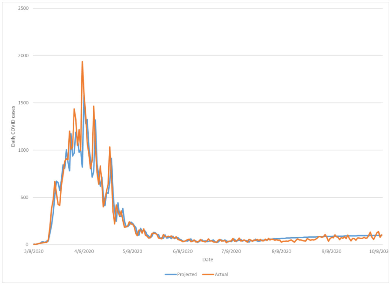
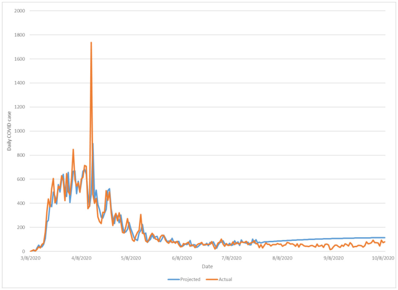
Modified VAR regression of NYC area COVID-19 caseload trends proves highly significant modelling capacity of observed patterns in longitudinal disease incidence (county R² range: 0.9221–0.9751, all p < 0.001). Predictively, VAR regression of daily caseload results at a county-wide level demonstrates considerable short-term forecasting fidelity (p < 0.001 at one-step ahead) with concurrent capacity for longer-term (tested 11-week period) inferences of consistent, reasonable upcoming patterns from latest (model data update) disease epidemiology.

Conclusions
In contrast to macroscopic variable-assumption projections, regionally-founded VAR modelling may substantially improve projection of short-term community disease burden, reduce potential for biostatistical error, as well as better model epidemiological effects resultant from intervention. Predictive VAR extrapolation of existing public health data at an interdependent regional scale may improve accuracy of current pandemic burden prognoses.
- novel coronavirus,
- COVID-19,
- vector autoregression,
- VAR,
- model,
- prediction,
- SIR,
- SARS-CoV-2
Citation: Aaron C Shang, Kristen E Galow, Gary G Galow. Regional forecasting of COVID-19 caseload by non-parametric regression: a VAR epidemiological model[J]. AIMS Public Health, 2021, 8(1): 124-136. doi: 10.3934/publichealth.2021010

Related Papers:

Abstract

Objectives

The COVID-19 pandemic (caused by SARS-CoV-2) has introduced significant challenges for accurate prediction of population morbidity and mortality by traditional variable-based methods of estimation. Challenges to modelling include inadequate viral physiology comprehension and fluctuating definitions of positivity between national-to-international data. This paper proposes that accurate forecasting of COVID-19 caseload may be best preformed non-parametrically, by vector autoregression (VAR) of verifiable data regionally.

Methods

A non-linear VAR model across 7 major demographically representative New York City (NYC) metropolitan region counties was constructed using verifiable daily COVID-19 caseload data March 12–July 23, 2020. Through association of observed case trends with a series of (county-specific) data-driven dynamic interdependencies (lagged values), a systematically non-assumptive approximation of VAR representation for COVID-19 patterns to-date and prospective upcoming trends was produced.

Results

Modified VAR regression of NYC area COVID-19 caseload trends proves highly significant modelling capacity of observed patterns in longitudinal disease incidence (county R² range: 0.9221–0.9751, all p < 0.001). Predictively, VAR regression of daily caseload results at a county-wide level demonstrates considerable short-term forecasting fidelity (p < 0.001 at one-step ahead) with concurrent capacity for longer-term (tested 11-week period) inferences of consistent, reasonable upcoming patterns from latest (model data update) disease epidemiology.

Conclusions

In contrast to macroscopic variable-assumption projections, regionally-founded VAR modelling may substantially improve projection of short-term community disease burden, reduce potential for biostatistical error, as well as better model epidemiological effects resultant from intervention. Predictive VAR extrapolation of existing public health data at an interdependent regional scale may improve accuracy of current pandemic burden prognoses.

Abbreviations

COVID-19/COVID

coronavirus disease 2019

SARS-CoV-2

Severe acute respiratory syndrome coronavirus 2

VAR

vector autoregression

NYC

New York City

S-I-R/SIR

susceptible, infectious, removed (immune) framework of compartmental disease modelling

SUQC

susceptible, unquarantined infected, quarantined infected, confirmed infected framework of compartmental disease modelling

AIC

Akaike Information Criteria

COVID+

confirmed positive COVID-19 case

MAE

mean absolute error

CDC

Centers for Disease Control and Prevention

Conflict of interest

All authors declare no conflicts of interest in this paper.

References

[1]	World Health Organization Coronavirus disease (‎‎COVID-19)‎‎: Weekly Epidemiological Report, 27 January 2021 (2021) .Available from: https://www.who.int/publications/m/item/weekly-epidemiological-update---27-january-2021.
[2]	Bai Y, Yao L, Wei T, et al. (2020) Presumed asymptomatic carrier transmission of COVID-19. JAMA 323: 1406-1407. doi: 10.1001/jama.2020.2565
[3]	Bastos ML, Tavaziva G, Abidi SK, et al. (2020) Diagnostic accuracy of serological tests for covid-19: systematic review and meta-analysis. BMJ 1: 370.
[4]	Roda WC, Varughese MB, Han D, et al. (2020) Why is it difficult to accurately predict the COVID-19 epidemic? Infect Dis Modell 5: 271-281. doi: 10.1016/j.idm.2020.03.001
[5]	Naudé W (2020) Artificial intelligence vs COVID-19: limitations, constraints and pitfalls. AI Soc 35.
[6]	Volpert V, Banerjee M, Petrovskii S (2020) On a quarantine model of coronavirus infection and data analysis. Math Modell Nat Phenom 15: 24. doi: 10.1051/mmnp/2020006
[7]	Zhao S, Chen H (2020) Modeling the epidemic dynamics and control of COVID-19 outbreak in China. Quant Biol 11: 1-9.
[8]	Shen CY (2020) A logistic growth model for COVID-19 proliferation: experiences from China and international implications in infectious diseases. Int J Infect Dis .
[9]	Elliott G, Stock JH (2001) Confidence intervals for autoregressive coefficients near one. J Econometrics 103: 155-181. doi: 10.1016/S0304-4076(01)00042-2
[10]	Hsiao WC, Huang HY, Ing CK (2018) Interval Estimation for a First-Order Positive Autoregressive Process. J Time Ser Anal 39: 447-467. doi: 10.1111/jtsa.12297
[11]	Branas CC, Rundle A, Pei S, et al. (2020) Flattening the curve before it flattens us: hospital critical care capacity limits and mortality from novel coronavirus (SARS-CoV2) cases in US counties. medRxiv .
[12]	Biswas K, Khaleque A, Sen P (2003) Covid-19 spread: Reproduction of data and prediction using a SIR model on Euclidean network. arXiv preprint arXiv:2003.07063 2020 Mar 16.
[13]	Postnikov EB (2020) Estimation of COVID-19 dynamics “on a back-of-envelope”: Does the simplest SIR model provide quantitative parameters and predictions? Chaos, Solitons Fractals 135: 109841. doi: 10.1016/j.chaos.2020.109841
[14]	Metcalf CJ, Lessler J (2017) Opportunities and challenges in modeling emerging infectious diseases. Science 357: 149-152. doi: 10.1126/science.aam8335
[15]	Funk S, Camacho A, Kucharski AJ, et al. (2018) Real-time forecasting of infectious disease dynamics with a stochastic semi-mechanistic model. Epidemics 22: 56-61. doi: 10.1016/j.epidem.2016.11.003
[16]	He ZL, Li JG, Nie L, et al. (2017) Nonlinear state-dependent feedback control strategy in the SIR epidemic model with resource limitation. Adv Differ Equ 2017: 1-8. doi: 10.1186/s13662-016-1057-2
[17]	Dubey B, Dubey P, Dubey US (2015) Dynamics of an SIR Model with Nonlinear Incidence and Treatment Rate. Appl Appl Math 10: 718-737.
[18]	Harjule P, Tiwari V, Kumar A (2021) Mathematical models to predict COVID-19 outbreak: An interim review. J Interdiscip Math 13: 1-26. doi: 10.1080/09720502.2020.1848316
[19]	Eker S (2020) Validity and usefulness of COVID-19 models. Humanit Soc Sci Commun 7: 1-5. doi: 10.1057/s41599-020-00553-4
[20]	Iwasaki A, Yang Y (2020) The potential danger of suboptimal antibody responses in COVID-19. Nat Rev Immunol 21: 1-3.
[21]	To KK, Tsang OT, Leung WS, et al. (2020) Temporal profiles of viral load in posterior oropharyngeal saliva samples and serum antibody responses during infection by SARS-CoV-2: an observational cohort study. Lancet Infect Dis .
[22]	Bertozzi AL, Franco E, Mohler G, et al. (2020) The challenges of modeling and forecasting the spread of COVID-19. arXiv preprint arXiv:2004.04741 .
[23]	Nakamura G, Grammaticos B, Deroulers C, et al. (2020) Effective epidemic model for COVID-19 using accumulated deaths. arXiv preprint arXiv:2007.02855 .
[24]	Bogg T, Milad E Slowing the Spread of COVID-19: Demographic, personality, and social cognition predictors of guideline adherence in a representative US sample (2020) .Available from: https://www.researchgate.net/publication/340427042_Slowing_the_Spread_of_COVID-19_Demographic_Personality_and_Social_Cognition_Predictors_of_Guideline_Adherence_in_a_Representative_US_Sample.
[25]	Dowd JB, Andriano L, Brazel DM, et al. (2020) Demographic science aids in understanding the spread and fatality rates of COVID-19. P Natl Acad Sci USA 117: 9696-9698. doi: 10.1073/pnas.2004911117

publichealth-08-01-010-s001.pdf

Reader Comments

Your name:*

Email:*
© 2021 the Author(s), licensee AIMS Press. This is an open access article distributed under the terms of the Creative Commons Attribution License (http://creativecommons.org/licenses/by/4.0)