Inspired by the COVID-19 pandemic, we build a large-scale epidemiological model that accounts for coordination between regions, each using travel restrictions in order to attempt to mitigate the spread of disease. There is currently a need for simulations of countries cooperating since travel restriction policies are typically taken without global considerations. It is possible, for instance, that a strategy which appears unfavorable to a region at some point during a pandemic might be best for containing the global spread, or that only by coordinating policies among several regions can a restriction strategy be truly effective. We use the formalism of hybrid automata to model the global disease spread among the coordinating regions. We model a connected network of coupled Susceptible-Exposed-Infected-Recovered (SEIR) models by considering a weighted directed graph with each node corresponding to a single region's disease model. The SEIR dynamics for each region admit terms for inter-regional travel determined by the graph's Laplacian that additionally accounts for travel restrictions between regions. The existence of an edge may change according to so-called guard conditions, which are triggered when the proportion of symptomatic infected individuals in a region reaches a critical value. Lastly, we run simulations in MATLAB of a global disease spreading among regions using automated travel restrictions and analyze the results.
Citation: Richard Carney, Monique Chyba, Taylor Klotz. Using hybrid automata to model mitigation of global disease spread via travel restriction[J]. Networks and Heterogeneous Media, 2024, 19(1): 324-354. doi: 10.3934/nhm.2024015
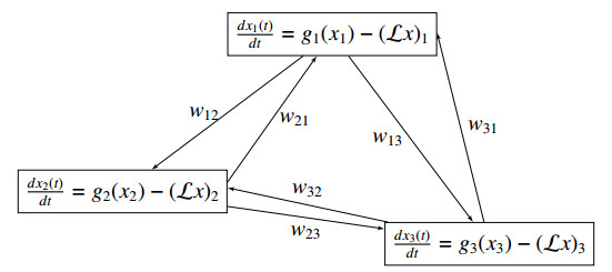
Inspired by the COVID-19 pandemic, we build a large-scale epidemiological model that accounts for coordination between regions, each using travel restrictions in order to attempt to mitigate the spread of disease. There is currently a need for simulations of countries cooperating since travel restriction policies are typically taken without global considerations. It is possible, for instance, that a strategy which appears unfavorable to a region at some point during a pandemic might be best for containing the global spread, or that only by coordinating policies among several regions can a restriction strategy be truly effective. We use the formalism of hybrid automata to model the global disease spread among the coordinating regions. We model a connected network of coupled Susceptible-Exposed-Infected-Recovered (SEIR) models by considering a weighted directed graph with each node corresponding to a single region's disease model. The SEIR dynamics for each region admit terms for inter-regional travel determined by the graph's Laplacian that additionally accounts for travel restrictions between regions. The existence of an edge may change according to so-called guard conditions, which are triggered when the proportion of symptomatic infected individuals in a region reaches a critical value. Lastly, we run simulations in MATLAB of a global disease spreading among regions using automated travel restrictions and analyze the results.

| [1] | S. Allred, M. Chyba, J. M. Hyman, Y. Mileyko, B. Piccoli, The Covid-19 pandemic evolution in hawai 'i and new jersey: A lesson on infection transmissibility and the role of human behavior, Predicting Pandemics in a Globally Connected World, Volume 1: Toward a Multiscale, Multidisciplinary Framework through Modeling and Simulation, Cham: Springer International Publishing, 2022,109–140. |
| [2] | Air Traffic By The Numbers, Federal Aviation Administration, United States Department of Transportation. Available from: https://www.faa.gov/air_traffic/by_the_numbers. |
| [3] | H. Duggal, M. Haddad, Visualising the global air travel industry, Al Jazeera. Available from: https://www.aljazeera.com/economy/2021/12/9/visualising-the-global-air-travel-industry-interactive. |
| [4] | F. R. Chung, Spectral graph theory, Conference Board of the mathematical sciences by the American Mathematical Society, Providence: American Mathematical Society, 1997. |
| [5] | C. Godsil, G. F. Royle, Algebraic Graph Theory, New York: Springer Science & Business Media, 2001. |
| [6] | A. Schaft, H. Schumacher, An introduction to hybrid dynamical systems, London: Springer, 2000. |
| [7] | R. Goebel, R. G. Sanfelice, A. R. Teel, Hybrid dynamical systems, IEEE Control Syst. Mag., 29 (2009), 28–93. https://doi.org/10.1109/MCS.2008.931718 |
| [8] |
R. Ross, An application of the theory of probabilities to the study of a priori pathometry.—Part I, Proceedings of the Royal Society of London. Series A, Containing papers of a mathematical and physical character, 92 (1916), 204–230. https://doi.org/10.1098/rspa.1916.0007 doi: 10.1098/rspa.1916.0007

|
| [9] | R. Ross, H. P. Hudson, An application of the theory of probabilities to the study of a priori pathometry.—Part II, Proceedings of the Royal Society of London. Series A, Containing papers of a mathematical and physical character, 93 (1917), 212–225. |
| [10] |
R. Ross, H. P. Hudson, An application of the theory of probabilities to the study of a priori pathometry.—Part III, Proceedings of the Royal Society of London. Series A, Containing papers of a mathematical and physical character, 93 (1917), 225–240. https://doi.org/10.1098/rspa.1917.0015 doi: 10.1098/rspa.1917.0015
|
| [11] | D. G. Kendall, Deterministic and stochastic epidemics in closed populations, in Proceedings of the third Berkeley symposium on mathematical statistics and probability, Berkeley: University of California Press, 1956,149–165. |
| [12] | W. O. Kermack, A. G. McKendrick, A contribution to the mathematical theory of epidemics, Proceedings of the royal society of london. Series A, Containing papers of a mathematical and physical character, 115 (1927), 700–721. |
| [13] |
P. Kunwar, O. Markovichenko, M. Chyba, Y. Mileyko, A. Koniges, T. Lee, A study of computational and conceptual complexities of compartment and agent based models, Netw. Heterog. Media., 17 (2022), 359–384. https://doi.org/10.3934/nhm.2022011 doi: 10.3934/nhm.2022011
|
| [14] |
R. Carney, M. Chyba, V. Y. Fan, P. Kunwar, T. Lee, I. Macadangdang, Y. Mileyko, Modeling variants of the covid-19 virus in hawai 'i and the responses to forecasting, AIMS Mathematics, 8 (2023), 4487–4523. https://doi.org/10.3934/math.2023223 doi: 10.3934/math.2023223
|
| [15] | J. Lygeros, S. Sastry, C. Tomlin, Hybrid systems: Foundations, advanced topics and applications, Berlin: Springer Verlag, 2012. |
| [16] | Port Authority Aviation Department, 2019 Annual Airport Traffic Report, Port Authority of New York and New Jersey. Available from: https://www.panynj.gov/content/dam/airports/statistics/statistics-general-info/annual-atr/ATR2019.pdf. |
| [17] | T. Crowfoot, World population just passed 8 billion. Here's what it means, World Economic Forum. Available from: https://www.weforum.org/agenda/2022/11/world-population-passes-8-billion-what-you-need-to-know. |


Figures(16) / Tables(7)
Richard Carney, Monique Chyba, Taylor Klotz. Using hybrid automata to model mitigation of global disease spread via travel restriction[J]. Networks and Heterogeneous Media, 2024, 19(1): 324-354. doi: 10.3934/nhm.2024015


 DownLoad: