Loading [MathJax]/jax/output/SVG/jax.js

A martingale formulation for stochastic compartmental susceptible-infected-recovered (SIR) models to analyze finite size effects in COVID-19 case studies

  • Received: 01 July 2021 Revised: 01 February 2022 Published: 30 March 2022
  • Primary: 60G51; Secondary: 35Q91

  • Deterministic compartmental models for infectious diseases give the mean behaviour of stochastic agent-based models. These models work well for counterfactual studies in which a fully mixed large-scale population is relevant. However, with finite size populations, chance variations may lead to significant departures from the mean. In real-life applications, finite size effects arise from the variance of individual realizations of an epidemic course about its fluid limit. In this article, we consider the classical stochastic Susceptible-Infected-Recovered (SIR) model, and derive a martingale formulation consisting of a deterministic and a stochastic component. The deterministic part coincides with the classical deterministic SIR model and we provide an upper bound for the stochastic part. Through analysis of the stochastic component depending on varying population size, we provide a theoretical explanation of finite size effects. Our theory is supported by quantitative and direct numerical simulations of theoretical infinitesimal variance. Case studies of coronavirus disease 2019 (COVID-19) transmission in smaller populations illustrate that the theory provides an envelope of possible outcomes that includes the field data.

    Citation: Xia Li, Chuntian Wang, Hao Li, Andrea L. Bertozzi. A martingale formulation for stochastic compartmental susceptible-infected-recovered (SIR) models to analyze finite size effects in COVID-19 case studies[J]. Networks and Heterogeneous Media, 2022, 17(3): 311-331. doi: 10.3934/nhm.2022009
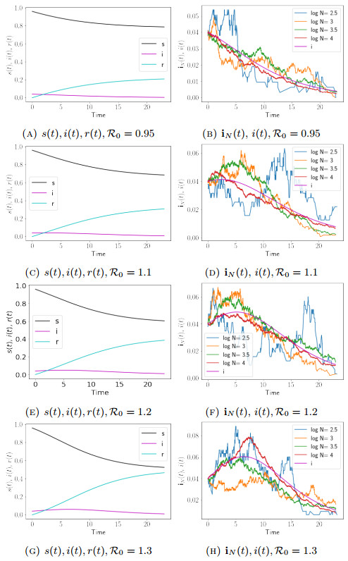
    Related Papers:

    [1] Yiyuan Qian, Haiming Song, Xiaoshen Wang, Kai Zhang . Primal-dual active-set method for solving the unilateral pricing problem of American better-of options on two assets. Electronic Research Archive, 2022, 30(1): 90-115. doi: 10.3934/era.2022005
    [2] Yiyuan Qian, Kai Zhang, Jingzhi Li, Xiaoshen Wang . Adaptive neural network surrogate model for solving the implied volatility of time-dependent American option via Bayesian inference. Electronic Research Archive, 2022, 30(6): 2335-2355. doi: 10.3934/era.2022119
    [3] Kaiyu Zhang . Sobolev estimates and inverse Hölder estimates on a class of non-divergence variation-inequality problem arising in American option pricing. Electronic Research Archive, 2024, 32(11): 5975-5987. doi: 10.3934/era.2024277
    [4] E. A. Abdel-Rehim . The time evolution of the large exponential and power population growth and their relation to the discrete linear birth-death process. Electronic Research Archive, 2022, 30(7): 2487-2509. doi: 10.3934/era.2022127
    [5] Shuaikang Wang, Yunzhi Jiang, Yongbin Ge . High-order compact difference methods for solving two-dimensional nonlinear wave equations. Electronic Research Archive, 2023, 31(6): 3145-3168. doi: 10.3934/era.2023159
    [6] Li Tian, Ziqiang Wang, Junying Cao . A high-order numerical scheme for right Caputo fractional differential equations with uniform accuracy. Electronic Research Archive, 2022, 30(10): 3825-3854. doi: 10.3934/era.2022195
    [7] Yan Dong . Local Hölder continuity of nonnegative weak solutions of inverse variation-inequality problems of non-divergence type. Electronic Research Archive, 2024, 32(1): 473-485. doi: 10.3934/era.2024023
    [8] Margarida Camarinha . A natural 4th-order generalization of the geodesic problem. Electronic Research Archive, 2024, 32(5): 3396-3412. doi: 10.3934/era.2024157
    [9] Haiyan Song, Fei Sun . A numerical method for parabolic complementarity problem. Electronic Research Archive, 2023, 31(2): 1048-1064. doi: 10.3934/era.2023052
    [10] Aya Selmoune, Zhiyuan Liu, Jinwoo Lee . To pay or not to pay? Understanding public acceptance of congestion pricing: A case study of Nanjing. Electronic Research Archive, 2022, 30(11): 4136-4156. doi: 10.3934/era.2022209
  • Deterministic compartmental models for infectious diseases give the mean behaviour of stochastic agent-based models. These models work well for counterfactual studies in which a fully mixed large-scale population is relevant. However, with finite size populations, chance variations may lead to significant departures from the mean. In real-life applications, finite size effects arise from the variance of individual realizations of an epidemic course about its fluid limit. In this article, we consider the classical stochastic Susceptible-Infected-Recovered (SIR) model, and derive a martingale formulation consisting of a deterministic and a stochastic component. The deterministic part coincides with the classical deterministic SIR model and we provide an upper bound for the stochastic part. Through analysis of the stochastic component depending on varying population size, we provide a theoretical explanation of finite size effects. Our theory is supported by quantitative and direct numerical simulations of theoretical infinitesimal variance. Case studies of coronavirus disease 2019 (COVID-19) transmission in smaller populations illustrate that the theory provides an envelope of possible outcomes that includes the field data.


    Assuming that the price of underlying assets satisfies the geometric Brownian motion, the Black-Scholes option pricing model was firstly proposed in 1973 which depends only on the risk-free interest rate and the volatility [1]. The Black-Scholes model quickly attracted a great deal of attention from the communities of both academic researcher and engineer. In order to improve the efficiency of the model and also fit the practical market, a sequence of option pricing models were proposed and studied, for instance, jump-diffusion model [2,3], stochastic volatility model [4,5] and the fractional option pricing models based on Lévy process including of finite moment log stable (FMLS) [6], KoBol [7,8] and CGMY [9] model.

    In order to solve the fractional option pricing models based on Lévy process, a number of numerical approaches were proposed and well studied in the past decades. Cont and Voltchkova [10] first presented a finite difference methods for solving the fractional European option pricing model driven by exponential Lévy process and studied the stability and convergence. Then, Cartea and del-Castillo-Negrete [11] rewrote FMLS, CGMY and KoBol option pricing models as a general fractional partial differential equation and studied the shifted Grünwald difference (SGD) formula for the numerical solution. Marom and Momoniat [12] further compared the numerical solutions of three fractional option pricing models based on Lévy process. Chen and Wang [13] developed a numerical scheme with second-order accuracy in both the spatial and time mesh size for pricing European and American option under a geometric Lévy process. Recently, Zhang et al. [14] constructed an implicit numerical scheme with second-order accuracy for FMLS model and used BiCGstab method to solve the discreted linear equations.

    As we known, exotic options play important roles and are widely used in the practical finance market [15]. However, it is a great challenge to obtain the solution for traditional numerical methods since the non-smooth payoffs usually lead to serious degradation in the convergence of the numerical schemes and result in inaccurate and discontinuous solution near the strike or barrier. For instance, the well known second-order implicit schemes, Crank-Nicolson method, are prone to spurious oscillations unless the time step size is small enough. To overcome this difficulty, Wade et al. [16] studied the Padé schemes to smooth the Crank-Nicolson scheme to get fourth-order schemes for pricing barrier European option models, see also [15,17,18,19] for the Padé schemes for different exotic option models.

    For the fractional exotic options under FMLS model, a class of fourth-order numerical schemes are presented and studied in this paper. We first discretize the fractional option pricing models with weighted and shifted Grünwald difference (WSGD) formula, which is of second-order accuracy in space direction. Then, by making use of the Padé schemes for the time direction, an L-stable and fourth-order accurate scheme is obtained. The convergence of the proposed numerical scheme is proved when the spatial discretization matrix is positive definite and has lower Hessenberg Toeplitz structure, without the assumption of the self-adjoint operator. The proposed method is adapted to be implemented on parallel processors by making use of partial fraction. Numerical experiments on digital option and barrier option are presented to verify the efficiency and accuracy of our numerical schemes.

    The structure of this paper is organized as follows. The weighted and shifted Grünwald difference schemes for space discretization is presented in Section 2. Time stepping schemes on Padé approximation and the implementations are presented in Section 3. We then analyze and prove the convergence of the numerical scheme in Section 4. Numerical experiments are given to show the accuracy and efficiency of the proposed schemes in Section 5. Finally, conclusions are drawn in Section 6.

    Denote St as the asset price at time t, the FMLS model [6] can be written as follow:

    V(x,t)t+(rν)V(x,t)x+νDαxV(x,t)=rV(x,t), (2.1)

    where V(x,t) is the price of the option at the time t before the expiry time T, x=lnSt, Dαx(1<α<2) is the left Riemann-Liouville derivative [20], ν=12σαsec(απ2), St is the price of underlying asset at time t, r is the risk free interest rate and σ is the volatility.

    In order to solve the FMLS model numerically, we first transform (2.1) into a forward problem by using the transformation t=Tt, and then drop for simplicity of the notation. Then we truncate the interval of x to a finite interval [Bd,Bu], and consider the following FMLS model for pricing European option

    V(x,t)t=(rν)V(x,t)x+νBdDαxV(x,t)rV(x,t),x(Bd,Bu),t(0,T], (2.2)

    where the left Riemann-Liouville derivative [20] is defined as

    BdDαxV(x,t)=1Γ(2α)d2dx2xBdV(η,t)(xη)α1dη,1<α<2,

    and the initial and boundary conditions are as follows:

    V(x,0)=v(x),BdxBu,V(Bd,t)=0,V(Bu,t)=B(t),0<t<T. (2.3)

    Let M and N be the number of the uniform discrete points in the space and time direction respectively, h=(BuBd)/M and τ=T/N be the corresponding step length. Define tj=jτ(j=0,1,2,,N),xi=Bd+ih(i=0,1,2,,M), then the discrete equation can be obtained. We discrete the first order derivative and α order left Riemann-Liouville fractional derivative by central difference scheme and weighted and shifted Grünwald difference (WSGD) scheme [21] respectively.

    The second-order WSGD scheme was first proposed by Tian et al. [21], which is a more general and flexible approach and independent on the changed fractional order. It is further applied into the numerical solution of time fractional sub-diffusion equation [22,23], as well as fractional Black-Schole equation in the FMLS model [14]. Recently Liu et al. [24] developed a class of second-order θ schemes based on the WSGD formula for solving the nonlinear fractional cable equation.

    Using WSGD scheme, the fractional derivative can be approximated as

    BdDαxV(xi,t)=1hαi+1k=0ω(α)kV(xik+1,t)+O(h2), (2.4)

    where

    {ω(α)0=α2g(α)0,ω(α)k=α2g(α)k+2α2g(α)k1g(α)0=1,g(α)k=(1α+1k)g(α)k1,k=1,2,.k=0g(α)k=0,g(α)k>0,k=0,2,3.g(α)1=α<0. (2.5)

    Denote Vji=V(xi,tj),Vj=(Vj1,Vj2,,VjM1)T,i=0,1,2,,M,j=0,1,2,,N, then the semidiscretization equation is given by

    Vt|(xi,tj)=(rν)Vji+1Vji12h+νhαi+1k=0ω(α)kVjik+1rVji, (2.6)

    where

    V0i=v(xi),i=1,2,,M1. (2.7)

    Denote ζ=νhα, ξ=rν2h, it leads to the following semi-equation

    Vt|(xi,tj)+AVj=fj,i=1,2,,M1, (2.8)

    where A=rIζBξC, B=[bij](M1)×(M1) defined by

    bij={ω(α)1,i=j,j=1,,M1,ω(α)2,i=j+1,j=1,,M2,ω(α)0,i=j1,j=2,,M1,ω(α)ij+1,ij2,j=1,,M3,0,otherwise, (2.9)

    C=tridiag{1,0,1} and fj=(0,0,,0,(ξ+ζω(α)0)(B(tj+1)+B(tj)). Since both the matrices B and C are Toeplitz matrices, the matrix A is also a Toeplitz matrix [25].

    In order to smooth the oscillations caused by the non-smooth payoff functions and improve the accuracy, we construct time stepping schemes with Padé approximation. The discretization (2.8) in space leads to the following system of initial value problem

    vt+Av=f(t),v(0)=v, (3.1)

    in a Hilbert space X, where v denotes the initial condition v(x) in (2.3). We assume the resolvent set ρ(A) (The points λ for which λIA has a bounded inverse in X comprise the resolvent set ρ(A) of A) satisfies, for some γ(0,π2) [26],

    ρ(A)ˉΣγ,Σγ:={zC:γ<|arg(z)|π,z0}, (3.2)

    Also, assume there exists C1 such that

    (zIA)1C|z|1,zΣγ. (3.3)

    The exact solution of (3.1) satisfies the following recurrence formula

    v(tj+1)=eτAv(tj)+τ10eτA(1η)f(tj+τη)dη, (3.4)

    where τ=T/N, j=0,1,2,,N1.

    Consider now its discrete analogue of the form

    vj+1=R(τA)vj+τmi=1Qi(τA)f(tj+siτ), (3.5)

    where {si}mi=1[0,1] are the the distinct numbers selected as integral points to approximate v(tj+1) in formula (3.4).

    The time discretization scheme (3.5) is accurate of order q in time which can be described as follow.

    Lemma 3.1. [26] The time discretization scheme (3.5) is accurate of order q if

    R(z)=ez+O(zq+1),as  z0, (3.6)

    and, for 0lq,

    mi=1sliQi(z)=l!(z)l+1(R(z)lj=0(z)jj!)+O(zql),as  z0, (3.7)

    or, equivalently,

    mi=1sliQi(z)=10slez(1s)ds+O(zql),as  z0. (3.8)

    It is shown in [26] that for the case m=q (m is the number of quadrature points and q is the accuracy of the scheme), the conditions of the Lemma 1 can be achieved by choosing the rational functions R(z) satisfying (3.6), selecting distinct real numbers, by Gaussian Quadrature, {Qi(z)}qi=1, and finally solving the system

    qi=1sliQi(z)=l!(z)l+1(R(z)lj=0(z)jj!),l=0,1,,q1. (3.9)

    This system (3.9) is of Vandermonde type (whose determinant is not zero), which gives the rational functions {Qi(z)}qi=1 as linear combinations of the terms on the right hand side of (3.9).

    For the case when the number of quadrature points m is less than the order of the scheme q, an alternative formula similar to (3.9) is given in [26]. The accuracy conditions are reformulated by defining

    Rl(z)=l!(z)l+1(R(z)lj=0(z)jj!)mi=1sliQi(z),l=0,1,,q1

    and requiring that

    Rl(z)=0,asz0,forl=0,1,,m1,

    and a moment condition

    10p(s)sjds=0,forj=0,,qm1. (3.10)

    on the quadrature points, with p(s)=mi=1(ssi). The formula to obtain the rational functions {Qi(z)}qi=1 in [26] is

    mi=1sliQi(z)=l!(z)l+1(R(z)lj=0(z)jj!),l=0,1,,m1. (3.11)

    For the rest of this chapter, we will use Padé approximation as R(z) above to constructe the high-order numerical scheme.

    Let Pn,m(z) and Qn,m(z) be two polynomials of degree n and m respectively, the (n+m) th order rational Padé approximation of the exponential function ez can be written as

    Rn,m(z)=Pn,m(z)Qn,m(z),

    where

    Pn,m(z)=nj=0(m+nj)!n!(m+n)!j!(nj)!(z)j,

    and

    Qn,m(z)=mj=0(m+nj)!m!(m+n)!j!(mj)!zj.

    The Padé approximation Rn,m(z) to the exponential function ez is of the order (n+m).

    Definition 3.1. The rational approximation Rn,m(z) of ez is said to be A-stable if |Rn,m(z)|<1 whenever (z)<0 and L-stable if in addition |Rn,m(z)|0 as (z).

    It is known from [27] that Rn,m(z)=ez+O(|z|m+n+1) as z0, and we consider the L-stable (0,2m)-Padé approximations and A-stable (m,m)-Padé approximations [28] for the exponential function ez.

    Here for practical purpose, we are particularly interested to the following A-stable and L-stable Padé approximation of ez respectively:

    R2,2(z)=112z+112z21+12z+112z2

    and

    R0,4(z)=11+z+12z2+16z3+124z4.

    Replace the matrix exponential eτA by (n,m) Padé approximation Rn,m(τA), the recurrence relation is approximated by

    Vj+1=Rn,m(τA)Vj+τ2i=1Q(i)n,m(τA)f(tj+siτ),j=0,1,2,,N1, (3.12)

    which is the fully discretization of (2.2). The {Q(i)n,m(z)}2i=1 are rational functions, which have same denominator as those Rn,m(z) and {si}2i=1 are the Gaussian points.

    Using the result of equation (3.11), we still have the same accuracy when we choose the corresponding Padé approximation

    2i=1sliQ(i)n,m(z)=l!(z)l+1(Rn,m(z)lj=0(z)jj!),l=0,1, (3.13)

    which is a linear system in Q(i)n,m(z) and could be solved easily since the matrix of the coefficients on the left is of Vandermonde's type.

    Consider the fourth order L-stable Padé approximation R0,4(z) with s1=336 and s2=3+36, the system reduces to

    Q(1)0,4(z)+Q(2)0,4(z)=1z(R0,4(z)1),s1Q(1)0,4(z)+s2Q(2)0,4(z)=1z2(R0,4(z)1+z). (3.14)

    Solving the Eq (3.14), it leads to the following fourth order schemes

    Vj+1=R0,4(τA)Vj+τQ(1)0,4(τA)g(tj+s1τ)+Q(2)0,4(τA)f(tj+s2τ),

    where

    Q(1)0,4(z)=12+(3312)z+(2324)z2+(1348)z31+z+12z2+16z3+124z4,Q(2)0,4(z)=12+(3+312)z+(2+324)z2+(1+348)z31+z+12z2+16z3+124z4.

    Both the schemes discussed above require to take inverse of higher order matrix polynomial which can cause computational difficulty due to higher power of matrix A.

    For overcoming this difficulty, Khaliq et al. [29], Gallopoulos and Saad [30] and references therein developed these schemes in a partial fraction decomposition (with complex arithmetic) that allows efficient and accurate computations on serial or parallel machines.

    The partial fraction form of the rational functions Rn,m(z) and {Q(i)n,m(z)}2i=1 requires us to consider two cases, n<m and n=m for subdiagonal and diagonal Padé schemes respectively.

    If n<m, then we have

    Rn,m(z)=q1j=1wjzci+2q1+q2j=q1+1(wjzci),Q(i)n,m(z)=q1j=1wijzci+2q1+q2j=q1+1(wijzci),i=1,2,

    and for the case n=m, the partial fraction form for Rn,m(z) and Q(i)n,m(z) is given by Gallopoulos and Saad [30]

    Rn,m(z)=(1)n+q1j=1wjzci+2q1+q2j=q1+1(wjzci),Q(i)n,m(z)=q1j=1wijzci+2q1+q2j=q1+1(wijzci),i=1,2,

    where Rn,m(z) as well as Q(i)n,m(z) have q1 real and 2q2 complex pole ci with q1+2q2=m, and wj=Rn,m(cj)Qn,m(cj) and wij=N(i)n,m(cj)D(i)n,m(cj).

    The polynomial N(i)n,m(z) and D(i)n,m(z) are the numerator and denominator of the function Q(i)n,m(z) respectively.

    The poles and weights for Rn,m(z) and Q(i)n,m(z) are:

    q1=0,q2=2,c1=0.270555768932292+2.50477590436244i,c2=1.729444231067690.888974376121862i,w1=0.541413348429154+0.248562520866115i,w2=0.541413348429182+1.58885918222330i,w11=0.2953739099586430.179575890979879i,w12=0.112361208066424+0.596907381204152i,w21=0.1742043074718740.023488268401115i,w22=0.508808394420345+0.002507912891072i.

    The algorithm becomes

    Vj+1=2(y1)+2(y2),

    where

    (τAc1I)y1=w1Vj+τw11f(tj+s1τ)+τw21f(tj+s2τ),(τAc2I)y2=w2Vj+τw12f(tj+s1τ)+τw22f(tj+s2τ),i=1,2, (3.15)

    which can be solved in parallel on two machines for speedup, or on a serial machine.

    In this section, we prove the convergence of the proposed scheme in the case that the spatial discretization matrix A is a lower Hessenberg Toeplitz matrix, without the assumption of a self-adjoint operator in [26].

    We begin with the proof of the positive definiteness of matrix A. The matrix A is positive definite if and only if its symmetric part W=(A+AT)/2 is positive definite [31], which means its eigenvalues are all positive.

    Theorem 4.1. Assume the fractional parameter α satisfying 1<α<2, the matrix A=rIζBξC defined in (2.8) as the following

    aij={ζω(α)1+r,i=j,j=1,,M1,ζω(α)2+ξ,i=j+1,j=1,,M2,ζω(α)0ξ,i=j1,j=2,,M1,ζω(α)ij+1,ij+2,j=1,,M3,0,otherwise, (4.1)

    is positive definite.

    Proof. Consider now the matrix W=[(ζBξC)+(ζBξC)T]/2 defined by

    wij={ζω(α)1,i=j,j=1,,M1,ζ(ω(α)0+ω(α)2)/2,|ij|=1,ζω(α)|ij|+1/2,|ij|2, (4.2)

    Use Gerschgorin Disk Theorem and note that wii=ζ(α+2)(α1)/2>0, we only need to prove it is row diagonally dominant and column diagonally dominant. It is clear that the ith and the (Mi1)th rows are the same. Without loss of generality, we choose 1iM12.

    For i=1, we have

    |w11|j1|w1j|=ζ2[2|ω(α)1||ω(α)0+ω(α)2|M1k=3|ω(α)k|]=ζ2[(1α4)(α+2)(α1)(α2g(α)2+g(α)2++g(α)M2+α2g(α)M1)]=ζ2[(α1)(α2+2)(g(α)2++g(α)M2+α2g(α)M1)]>ζ2[(α1)(α2+2)k=2g(α)k]=ζ2[(α1)(α2+2)(α1)]=ζ2(α1)(α2+1)>0.

    For i=2,3,,M12, using the properties in (2.5), we have

    |wii|j1|wij|=ζ2[2|ω(α)1|2|ω(α)0+ω(α)2|2ik=3|ω(α)k|Mik=i+1|ω(α)k|]=ζ2[(2α)(α+2)(α1)22ik=3|ω(α)k|Mik=i+1|ω(α)k|]>ζ2[(2α)(α+2)(α1)22Mik=3|ω(α)k|]=ζ2[(2α)(α+2)(α1)22(α2g(α)2+g(α)2++g(α)M2+α2g(α)M1)]=ζ2[2(α1)2Mik=3g(α)k]>ζ2[2(α1)2k=2g(α)k]=ζ2[2(α1)2(α1)]=0.

    Therefore, the matrix W is row diagonal dominant. Because of its Toeplitz structure, it is column diagonally dominant as well, and thus the matrix A is positive definite.

    Assume the function R() is the L-stable (0,2m)-Padé approximation of order q in (3.6), and v is the initial condition in (3.1), then the convergence of the scheme is established in the following two theorems.

    Theorem 4.2. Assume that A defined in (3.1) and satisfying (3.2) and (3.3) is diagonalizable. For the R() and q>0 in (3.6), there exists a constant C>0 such that for n>1

    (etnARn(τA))vCτqv,vRM1. (4.3)

    Proof. Let A have eigenvalues {λi}M1i=1 and corresponding orthonormal eigenvectors {wi}M1i=1. Suppose v=M1j=1αjwj, then we have

    etnAv=M1j=1αjeλjtnwj,

    and

    Rn(τA)v=M1j=1αjRn(τλj)wj.

    It follows that

    (etnARn(τA))v2=M1j=1α2j|enτλjRn(τλj)|2.

    Using the identity anbn=(ab)n1j=0ajbnj1, it follows that

    |enτλjRn(τλj)|=|(eτλjR(τλj))n1j=0(eτjλjRnj1(τλj))|=|(τλj)q+1n1j=0(eτjλjRnj1(τλj))|.

    Without the confusion, we will reuse the constant C from line to line. From Theorem 4.1 we know that A is positive definite, thus (λj)>0,j=1,2,M1. For any integer k0 and l>0, there exists a constant C such that

    |(τλj)keτlλj|C, (4.4)

    We also find there exists 0<c<1 such that |R(z)|ecz for (0, 4)-Padé scheme, thus we have the following bound

    |enτλjRn(τλj)|Cnτq+1ec(n1)τλ=Cτq.

    Therefore,

    (etnARn(τA))v2Cτ2qM1j=1α2j=Cτ2qv2,

    and the proof is complete.

    Use the results of Theorem 4.2, and define the spaces ˙Hs=D(As/2) in [26] with the norm as following

    |v|s=(Asv,v)1/2=As/2v=(M1j=1λsj(v,wj)2)1/2,

    we complete the proof of the convergence in the following theorem.

    Theorem 4.3. Suppose that f(l)(t)˙H2q2l for l<q and t0, then there exists a constant C such that

    vnv(tn)Cτq(v+tnq1l=0sups<tn|f(l)(s)|2q2l+tn0f(q)ds), (4.5)

    i.e., the time discretization scheme (3.5) is accurate of order q.

    Proof. The error En=vnv(tn), for n2, can be written as:

    En=(Rn(τA)E(tn))vEn0+τn1j=0(Rnj1(τA)Rkf(tj)E(ttj1)Ikf(tj))Enq, (4.6)

    where E(t)=etA,

    Ikf(tj)=10E(τsτ)f(tj+sτ)ds,Rkf(tj)=mi=1Qi(τA)f(tj+siτ).

    The error term En0 can be approximated by the established result from Theorem 4.2 as follows:

    En0=(etnARn(τA))vCτqv. (4.7)

    After inserting the term Rnj1(τA)Ikf(tj) in the error term Enq and rearranging its terms, it can be derived as

    Enq=τn1j=0(Rnj1(τA)E(tnj1))Ikf(tj)En1+τn1j=0Rnj1(τA)(RkIk)f(tj)En2. (4.8)

    Following the approach given in [26], we have the following estimate for En1 and En2,

    En1Cτqtn0|f|2qds, (4.9)

    which is bounded by the right hand side of (4.5). Also

    En2n1j=0Cτq+1q1j=0|f(l)(tj)|2q2l+Cτqn10tj+1tjf(q)ds. (4.10)

    Since Eq (4.9) can be incorporated into the right hand side of (4.10), we obtain the following estimate for the main scheme:

    Enqn1j=0Cτq+1q1j=0|f(l)(tj)|2q2l+Cτqn10tj+1tjf(q)ds,Cτqtnq1l=0sups<tn|f(l)(s)|2q2l+Cτqtn0f(q)ds. (4.11)

    Combining (4.7) and (4.11), it leads to

    EnEn0+EnqCτq(v+tnq1l=0sups<tn|f(l)(s)|2q2l+tn0f(q)ds), (4.12)

    which completes the proof.

    In this section, numerical performance of different Padé schemes compared with the Crank-Nicolson scheme is given for the numerical solution of both fractional digital options and fractional barrier options.

    Since the non-smooth payoffs of fractional exotic options usually result in inaccurate and discontinuous solution, or serious errors when estimating the hedging parameters, e.g., Delta, Vega and Gamma values, we compare the price of the options under different schemes, as well as the Delta [16,32,33], which is the rate of change of the option value with respect to the asset price and can be approximated in the following way:

    VS|Si=1exiVx|xiV(xi+1,t)V(xi1,t)2hexi.

    The order of the numerical scheme is defined as

    Order=logτ2τ1Vτ2(,0)V(,0)Vτ1(,0)V(,0),

    where V(,0) denotes the exact solution at t=0 and Vτ(,0) denotes the numerical solution with time step τ at t=0. In our experiments, the exact solution V(,0) is approximated by the numerical solution using a dense mesh with M=N=8192 and we set τ2/τ1=2 to obtain the convergence order.

    Example 5.1. Consider a fractional digital call option pricing model as follows

    {V(x,t)t+(rν)V(x,t)x+νBdDαxV(x,t)=rV(x,t),(x,t)(Bd,Bu)×(0,T),V(Bd,t)=0,V(Bu,t)=50er(Tt),t[0,T),V(x,T)=v(x),x(Bd,Bu),

    where α=1.5,r=0.05,σ=0.25,Bu=ln100,Bd=ln0.1,T=1,K=50 and ν=12σαsecαπ2 where the payoff function is

    v(x)={50,lnK<x<Bu,25,x=lnK,0,Bd<x<lnK.,

    where we take the average of playoff at x=lnK from mathematical viewpoint to restore the discontinuity in the payoff [15].

    In Figures 13, the surfaces of the price and the corresponding Delta value of the fractional European digital option are plotted for the Crank-Nicolson, (2, 2)-Padé and (0, 4)-Padé schemes respectively when N=16 and M=4096.

    Figure 1.  The price and Delta of digital option using the Crank-Nicolson scheme.
    Figure 2.  The price and Delta of digital option using the (2, 2)-Padé scheme.
    Figure 3.  The price and Delta of digital option using the (0, 4)-Padé scheme.

    From Figures 13, it is observed that the second-order Crank–Nicolson method suffers from oscillations with non-smooth payoff function while the (0, 4)-Padé scheme can provide reliable and smooth option values and Delta value with little oscillation.

    The reason for the oscillation phenomenon at the strike price is that the time discretization grids are coarse [33,34]. One possible remedy is reducing the discrete step size in time direction or local mesh refinement strategy [35,36], which would highly increase the computational time. Here, the (0, 4)-Padé scheme could obtain the best accuracy cheaply and smooth the oscillations with relative less discrete points.

    In Tables 13, we list the error of the numerical solution in L2 and L norm, as well as the corresponding order for the Crank-Nicolson scheme, (2, 2)-Padé and (0, 4)-Padé respectively when τ is varying and M=8192.

    Table 1.  The numerical results of digital option with the Crank-Nicolson scheme.
    N τ Vτ(,0)V(,0)2 Order Vτ(,0)V(,0) Order
    8 0.12500000 51.4645 *** 27.0184 ***
    16 0.06250000 27.4790 0.9052 19.2316 0.4905
    32 0.03125000 10.3013 1.4155 6.1728 1.6395
    64 0.01562500 1.0048 3.3578 4.9171×101 3.6500
    128 0.00781250 3.4284×10³ 8.1952 2.2191×10⁴ 11.1136

     | Show Table
    DownLoad: CSV
    Table 2.  The numerical results of digital option with the (2, 2)-Padé scheme.
    N τ Vτ(,0)V(,0)2 Order Vτ(,0)V(,0) Order
    8 0.12500000 31.7954 *** 21.3352 ***
    16 0.06250000 13.3594 1.2510 9.0302 1.2404
    32 0.03125000 2.0437 2.7086 1.3213 2.7728
    64 0.01562500 5.1328×10³ 8.6372 2.7977×10³ 8.8835
    128 0.00781250 7.4134×10⁸ 16.0793 4.8969×10⁹ 19.1239

     | Show Table
    DownLoad: CSV
    Table 3.  The numerical results of digital option with the (0, 4)-Padé scheme.
    N τ Vτ(,0)V(,0)2 Order Vτ(,0)V(,0) Order
    8 0.12500000 1.7217×10² *** 1.1203×10³ ***
    16 0.06250000 1.3686×10³ 3.6530 9.0190×10⁵ 3.6348
    32 0.03125000 9.7572×10⁵ 3.8101 8.1591×10⁶ 3.4665
    64 0.01562500 7.0293×10⁶ 3.7950 1.8366×10⁶ 2.1514
    128 0.00781250 7.8313×10⁷ 3.1661 3.8539×10⁷ 2.2526

     | Show Table
    DownLoad: CSV

    From Tables 13, it is seen that the numerical results of digital option with both (2, 2)-Padé scheme and (0, 4)-Padé scheme have fourth-order accuracy, which is much better than those of the Crank-Nicolson scheme.

    In Figure 4, we plot the curves of option price and the corresponding Delta value versus the price of the asset when t=0 for the Crank-Nicolson, (2, 2)-Padé and (0, 4)-Padé scheme respectively.

    Figure 4.  The price and Delta of Digital option at time t=0 using different schemes.

    From Figure 4, it is further confirmed that the (0, 4)-Padé scheme can significantly reduce the oscillations of the solution near the strike price and smooth both the price of option and the Delta value, compared with the Crank-Nicolson and (2, 2)-Padé schemes. It is possibly because of (0, 4)-Padé scheme is a high order scheme, so that it can quickly converges to the exact solution with less time layer.

    Example 5.2. Consider a fractional barrier put option pricing model as follows

    {V(x,t)t+(rν)V(x,t)x+νBdDαxV(x,t)=rV(x,t),(x,t)(Bd,Bu)×(0,T),V(Bu,t)=V(Bd,t)=0,t[0,T),V(x,T)=v(x),x(Bd,Bu),

    where α=1.5,r=0.05,σ=0.25,Bu=ln100,Bd=ln0.1,T=1,K=50,E=20 and ν=12σαsecαπ2. The payoff function is

    v(x)={max{Kex,0},lnE<xBu,0,Bd<xlnE.

    In Figures 57, the price surfaces of the fractional barrier put option and the corresponding Delta value are plotted for the Crank-Nicolson, (2, 2)-Padé and (0, 4)-Padé schemes respectively when N=16 and M=4096.

    Figure 5.  The price and Delta of barrier option using the Crank-Nicolson scheme.
    Figure 6.  The price and Delta of barrier option using the (2, 2)-Padé scheme.
    Figure 7.  The price and Delta of barrier option using the (0, 4)-Padé scheme.

    From Figures 57, it is observed that the option price and Delta value of the Crank–Nicolson method still suffer from serious oscillations near the barrier while those of the (0, 4)-Padé scheme provide the best approximate results.

    It is also seen that though the (2, 2)-Padé scheme makes use of the same interpolation points with the (0, 4)-Padé scheme, the price of option and Delta values of the (2, 2)-Padé scheme still oscillate near the barrier.

    Moreover, in Figure 8, we plot the curves of option price and the corresponding Delta value versus the asset price when t=0 for the Crank-Nicolson, (2, 2)-Padé and (0, 4)-Padé scheme respectively.

    Figure 8.  The price and Delta of barrier option at time t=0 using different schemes.

    From Figure 8, it is further verified that the (0, 4)-Padé scheme is the best one, which can significantly reduce the oscillations of the option price and the Delta value near the barrier.

    In Tables 46, the error of the numerical solution in L2 and L norm, as well as the corresponding order for the Crank-Nicolson, (2, 2)-Padé and (0, 4)-Padé schemes are listed respectively when τ is varying and M=8192.

    Table 4.  The numerical results of barrier option with the Crank-Nicolson scheme.
    N τ Vτ(,0)V(,0)2 Order Vτ(,0)V(,0) Order
    8 0.12500000 33.7205 *** 17.8600 ***
    16 0.06250000 19.9914 0.7542 14.8495 0.2663
    32 0.03125000 8.8330 1.1784 7.7376 0.9405
    64 0.01562500 9.9060×101 3.1565 7.8221×101 3.3063
    128 0.00781250 2.1208×10³ 8.8676 2.3627×10⁴ 11.6929

     | Show Table
    DownLoad: CSV
    Table 5.  The numerical results of barrier option with the (2, 2)-Padé scheme.
    N τ Vτ(,0)V(,0)2 Order Vτ(,0)V(,0) Order
    8 0.12500000 22.5121 *** 15.7317 ***
    16 0.06250000 11.0447 1.0274 9.6167 0.7101
    32 0.03125000 1.9755 2.4831 1.4823 2.6977
    64 0.01562500 5.2250×10³ 8.5626 3.1998×10³ 8.8556
    128 0.00781250 4.4324×10⁸ 16.8470 2.9549×10⁹ 20.0465

     | Show Table
    DownLoad: CSV
    Table 6.  The numerical results of barrier option with the (0, 4)-Padé scheme.
    N τ Vτ(,0)V(,0)2 Order Vτ(,0)V(,0) Order
    8 0.12500000 1.0414×10² *** 6.7754×10⁴ ***
    16 0.06250000 8.2617×10⁴ 3.6559 5.4547×10⁵ 3.6347
    32 0.03125000 5.8268×10⁵ 3.8257 3.8767×10⁶ 3.8146
    64 0.01562500 3.8786×10⁶ 3.9091 2.5746×10⁷ 3.9124
    128 0.00781250 3.1080×10⁷ 3.6415 1.5452×10⁸ 4.0584

     | Show Table
    DownLoad: CSV

    From Tables 46, it is observed that the price of the digital option with both (2, 2)-Padé scheme and (0, 4)-Padé scheme can achieve the fourth-order accuracy, while the results of the (0, 4)-Padé scheme are more accurate than those of the (2, 2)-Padé scheme.

    Example 5.3. Consider a fractional double barrier call option pricing model as follows

    {V(x,t)t+(rν)V(x,t)x+νBdDαxV(x,t)=rV(x,t),(x,t)(Bd,Bu)×(0,T),V(Bu,t)=V(Bd,t)=0,t[0,T),V(x,T)=v(x),x(Bd,Bu),

    where α=1.5,r=0.05,σ=0.25,Bu=ln100,Bd=ln0.1,T=1,K=20,E1=40,E2=70 and ν=12σαsecαπ2. The payoff function is

    v(x)={max{exK,0},lnE1<xlnE2,0,Bd<xlnE1,lnE2x<Bu.

    In Figures 911, the price surfaces of the fractional double barrier call option and the corresponding Delta value are drawn for the Crank-Nicolson, (2, 2)-Padé and (0, 4)-Padé schemes respectively with N=16 and M=2048.

    Figure 9.  The price and Delta of double barrier option using the Crank-Nicolson scheme.
    Figure 10.  The price and Delta of double barrier option using the (2, 2)-Padé scheme.
    Figure 11.  The price and Delta of double barrier option using the (0, 4)-Padé scheme.

    From Figures 911, it is observed that both the Crank–Nicolson and (2, 2)-Padé schemes suffer from spurious oscillations near the barrier while (0, 4)-Padé approximation provides reliable option values and smooth Delta value.

    In Figure 12, we plot the curves of option price and the corresponding Delta value versus the asset price when t=0 for Crank-Nicolson, (2, 2)-Padé and (0, 4)-Padé scheme respectively.

    Figure 12.  The price and Delta of double barrier option at time t=0 using different schemes.

    From Figure 12, it is further confirmed that the (0, 4)-Padé scheme can significantly reduce the oscillation of the price of the option near the barrier and smooth the corresponding Delta value.

    In Tables 79, the error of the numerical solution in L2 and L norm, as well as the corresponding order for the Crank–Nicolson, (2, 2)-Padé and (0, 4)-Padé schemes are listed respectively when τ is varying and M=8192.

    Table 7.  The numerical results of double barrier option with the Crank–Nicolson scheme.
    N τ Vτ(,0)V(,0)2 Order Vτ(,0)V(,0) Order
    8 0.12500000 60.6264 *** 29.9147 ***
    16 0.06250000 35.9440 0.7542 24.8172 0.2695
    32 0.03125000 15.8816 1.1784 12.9186 0.9419
    64 0.01562500 1.7811 3.1565 1.3060 3.3062
    128 0.00781250 3.6030×10³ 8.9493 3.7585×10⁴ 11.7628

     | Show Table
    DownLoad: CSV
    Table 8.  The numerical results of double barrier option with the (2, 2)-Padé scheme.
    N τ Vτ(,0)V(,0)2 Order Vτ(,0)V(,0) Order
    8 0.12500000 40.4761 *** 26.3017 ***
    16 0.06250000 19.8581 1.0273 16.0588 0.7118
    32 0.03125000 3.5519 2.4831 2.4759 2.6974
    64 0.01562500 9.3945×10³ 8.5626 5.3429×10³ 8.8561
    128 0.00781250 7.9967×10⁸ 16.8421 5.0636×10⁹ 20.0090

     | Show Table
    DownLoad: CSV
    Table 9.  The numerical results of double barrier option with the (0, 4)-Padé scheme.
    N τ Vτ(,0)V(,0)2 Order Vτ(,0)V(,0) Order
    8 0.12500000 1.9302×10² *** 1.0964×10³ ***
    16 0.06250000 1.5287×10³ 3.6584 8.8458×10⁵ 3.6316
    32 0.03125000 1.0763×10⁴ 3.8281 6.3074×10⁶ 3.8099
    64 0.01562500 7.1519×10⁶ 3.9117 4.3025×10⁷ 3.8738
    128 0.00781250 5.1858×10⁷ 3.7857 3.6863×10⁸ 3.5449

     | Show Table
    DownLoad: CSV

    From Tables 79, it is seen that the numerical price of the fractional double barrier call option for both (2, 2)-Padé scheme and (0, 4)-Padé scheme can achieve fourth-order accuracy while the numerical results of the Crank–Nicolson scheme only obtains the second-order accuracy. Among the three schemes, the (0, 4)-Padé scheme is the most accurate one, which requires less discrete points than the other two schemes to achieve the same accuracy.

    A class of fourth order Padé schemes for pricing fractional exotic options under FMLS model are proposed and studied, which make use of the 2nd-order weighted and shifted Grünwald difference scheme in space direction and the 4th-order Padé schemes in time direction. The convergence of the Padé schemes are proved in detailed under the FMLS model. Numerical experiments on fractional digital option and fractional barrier options are given to verify the 4th-order precision, and show that the (0, 4)-Padé scheme can significantly reduce the oscillations of the solution near the strike price or barrier, smooth the Delta value and save the computational time.

    The authors are very grateful to the referees for their constructive comments and valuable suggestions, which greatly improved the original manuscript of the paper. This work is supported by the National Natural Science Foundation of China (No. 11971354).

    The authors declare there is no conflicts of interest.


    [1]

    L. J. S. Allen, An introduction to stochastic epidemic models, In Mathematical Epidemiology, Lecture Notes in Math., 1945 (2008), 81–130.

    [2] (2011) An Introduction to Stochastic Processes with Applications to Biology. Boca Raton, FL: CRC Press.
    [3]

    L. J. Allen and E. J. Allen, A comparison of three different stochastic population models with regard to persistence time, Theoretical Population Biology, 64 (2003), 439–449, https://www.sciencedirect.com/science/article/pii/S0040580903001047.

    [4] On SIR-models with Markov-modulated events: Length of an outbreak, total size of the epidemic and number of secondary infections. Discrete Contin. Dyn. Syst. Ser. B (2018) 23: 2153-2176.
    [5]

    D. Applebaum, Lévy Processes and Stochastic Calculus, vol. 116 of Cambridge Studies in Advanced Mathematics, 2nd edition, Cambridge Studies in Advanced Mathematics, 116. Cambridge University Press, Cambridge, 2009.

    [6]

    P. Azimi, Z. Keshavarz, J. G. Cedeno Laurent, B. Stephens and J. G. Allen, Mechanistic transmission modeling of COVID-19 on the diamond princess cruise ship demonstrates the importance of aerosol transmission, Proceedings of the National Academy of Sciences, 118 (2021).

    [7]

    N. T. J. Bailey, The Mathematical Theory of Infectious Diseases and Its Applications, 2nd edition, Hafner Press [Macmillan Publishing Co., Inc.], New York, 1975.

    [8] The critical community size for measles in the united states. Journal of the Royal Statistical Society: Series A (General) (1960) 123: 37-44.
    [9] A review of seir-d agent-based model. Distributed Computing and Artificial Intelligence, 16th International Conference, Special Sessions (2019) 1004: 133-140.
    [10]

    T. Belin, A. Bertozzi, N. Chaudhary, T. Graves, J. Guterman, M. C. Jarashow, R. J. Lewis, J. Marion, F. Schoenberg, M. Shah, J. Tolles, E. Traub, K. Viele and F. Wu, Projections of Hospital-based Healthcare Demand due to COVID-19 in Los Angeles County May 24, 2021, 2021, http://file.lacounty.gov/SDSInter/dhs/1107440_COVID-19ProjectionPublicUpdateLewis05.24.21English.pdf.,

    [11]

    A. L. Bertozzi, E. Franco, G. Mohler, M. B. Short and D. Sledge, The challenges of modeling and forecasting the spread of COVID-19, Proc. Natl. Acad. Sci., 117 (2020), 16732–16738, https://www.pnas.org/content/117/29/16732.

    [12] Martingale estimation functions for discretely observed diffusion processes. Bernoulli (1995) 1: 17-39.
    [13] (2002) Stochastic Integration with Jumps. Cambridge: Encyclopedia of Mathematics and its Applications, 89. Cambridge University Press.
    [14] Gaussian process approximations for fast inference from infectious disease data. Math. Biosci. (2018) 301: 111-120.
    [15] Refined stability thresholds for localized spot patterns for the Brusselator model in R2. European J. Appl. Math. (2019) 30: 791-828.
    [16]

    K. L. Chung and R. J. Williams, Introduction to Stochastic Integration, 2nd edition, Modern Birkhäuser Classics, Birkhäuser/Springer, New York, 2014.

    [17] Nonparametric estimation for stochastic differential equations with random effects. Stochastic Process. Appl. (2013) 123: 2522-2551.
    [18]

    P. Cruises, Princess cruise lines (2020) Diamond Princess updates, 2021, https://www.princess.com/news/notices_and_advisories/notices/diamond-princess-update.html.

    [19] An interactive web-based dashboard to track COVID-19 in real time. The Lancet Infectious Diseases (2020) 20: 533-534.
    [20] (1996) Stochastic Calculus. Boca Raton, FL: A practical introduction. Probability and Stochastics Series. CRC Press.
    [21]

    R. Durrett, Essentials of Stochastic Processes, Springer Texts in Statistics, Springer-Verlag, New York, 1999.

    [22]

    R. Durrett, Probability Models for DNA Sequence Evolution, Probability and its Applications (New York), Springer-Verlag, New York, 2002.

    [23]

    S. N. Ethier and T. G. Kurtz, Markov Processes: Characterization and Convergence., Wiley Series in Probability and Mathematical Statistics: Probability and Mathematical Statistics, John Wiley & Sons, Inc., New York, 1986.

    [24]

    N. M. Ferguson, D. Laydon, G. Nedjati-Gilani, N. Imai, K. Ainslie, M. Baguelin, S. Bhatia, A. Boonyasiri, Z. Cucunubá, G. Cuomo-Dannenburg, A. Dighe, I. Dorigatti, H. Fu, K. Gaythorpe, W. Green, A. Hamlet, W. Hinsley, L. C. Okell, S. v. Elsland, H. Thompson, R. Verity, E. Volz, H. Wang, Y. Wang, P. G. Walker, C. Walters, P. Winskill, C. Whittaker, C. A. Donnelly, S. Riley and A. C. Ghani, Impact of non-pharmaceutical interventions (NPIs) to reduce COVID-19 mortality and healthcare demand, Report 9, Imperial College COVID-19 Response Team, Imperial College London, London, United Kingdom, 2020.

    [25] A general method for numerically simulating the stochastic time evolution of coupled chemical reactions. J. Comput. Phys. (1976) 22: 403-434.
    [26] The linear stability of symmetric spike patterns for a bulk-membrane coupled Gierer-Meinhardt model. SIAM J. Appl. Dyn. Syst. (2019) 18: 729-768.
    [27]

    M. Z. Guo, G. C. Papanicolaou and S. R. S. Varadhan, Nonlinear diffusion limit for a system with nearest neighbor interactions, Comm. Math. Phys., 118 (1988), 31–59, http://projecteuclid.org/euclid.cmp/1104161907.

    [28] Turbulent energy density in scale space for inhomogeneous turbulence. J. Fluid Mech. (2018) 842: 532-553.
    [29] Geometric decomposition of the conformation tensor in viscoelastic turbulence. J. Fluid Mech. (2018) 842: 395-427.
    [30]

    S. W. He, J. G. Wang and J. A. Yan, Semimartingale Theory and Stochastic Calculus, Kexue Chubanshe (Science Press), Beijing; CRC Press, Boca Raton, FL, 1992.

    [31]

    P. G. Hoel, S. C. Port and C. J. Stone, Introduction to Stochastic Processes, The Houghton Mifflin Series in Statistics, Houghton Mifflin Co., Boston, Mass., 1972.

    [32] Estimating large-scale structures in wall turbulence using linear models. J. Fluid Mech. (2018) 842: 146-162.
    [33] Assessing the variability of stochastic epidemics. Mathematical Biosciences (1991) 107: 209-224.
    [34]

    V. Isham, Stochastic models for epidemics with special reference to AIDS, Ann. Appl. Probab., 3 (1993), 1–27, http://links.jstor.org/sici?sici=1050-5164(199302)3:1<1:SMFEWS>2.0.CO;2-4&origin=MSN.

    [35]

    V. Isham, Stochastic models for epidemics, In Celebrating Statistics, Oxford Statist. Sci. Ser., Oxford Univ. Press, Oxford, 33 (2005), 27–54.

    [36]

    J. Jiménez, Coherent structures in wall-bounded turbulence, J. Fluid Mech., 842 (2018), P1,100.

    [37]

    S. Karlin and H. M. Taylor, A Second Course in Stochastic Processes, Academic Press, Inc. [Harcourt Brace Jovanovich, Publishers], New York-London, 1981.

    [38]

    W. O. Kermack, A. G. McKendrick and G. T. Walker, A contribution to the mathematical theory of epidemics, Proceedings of the Royal Society of London. Series A, Containing Papers of a Mathematical and Physical Character, 115 (1927), 700–721, https://royalsocietypublishing.org/doi/abs/10.1098/rspa.1927.0118.

    [39] Hydrodynamics and large deviation for simple exclusion processes. Comm. Pure Appl. Math. (1989) 42: 115-137.
    [40]

    C. Kipnis and C. Landim, Scaling Limits of Interacting Particle Systems, Springer-Verlag, Berlin, 1999.

    [41]

    T. Kolokolnikov, M. Ward, J. Tzou and J. Wei, Stabilizing a homoclinic stripe, Philos. Trans. Roy. Soc. A, 376 (2018), 20180110, 13 pp.

    [42] Pattern formation in a reaction-diffusion system with space-dependent feed rate. SIAM Rev. (2018) 60: 626-645.
    [43] Novel moment closure approximations in stochastic epidemics. Bull. Math. Biol. (2005) 67: 855-873.
    [44]

    H. Kunita, Lectures on Stochastic Flows and Applications, Springer-Verlag, Berlin, 1986.

    [45] Comparison of three sis epidemic models: Deterministic, stochastic and uncertain. Journal of Intelligent & Fuzzy Systems (2018) 35: 5785-5796.
    [46]

    T. M. Liggett, Interacting Markov processes, In Biological Growth and Spread (Proc. Conf., Heidelberg, 1979), 38 (1980), 145–156.

    [47]

    T. M. Liggett, Interacting Particle Systems, Springer-Verlag, New York, 1985.

    [48]

    T. M. Liggett, Continuous Time Markov Processes, American Mathematical Society, Providence, RI, 2010.

    [49] Approximation methods for analyzing multiscale stochastic vector-borne epidemic models. Math. Biosci. (2019) 309: 42-65.
    [50]

    A. L. Lloyd, Realistic distributions of infectious periods in epidemic models: Changing patterns of persistence and dynamics, Theoretical Population Biology, 60 (2001), 59–71, http://www.sciencedirect.com/science/article/pii/S0040580901915254.

    [51]

    S. McMiNN, R. Talbot and J. ENG, America's 200,000 COVID-19 deaths: Small cities and towns bear a growing share, https://www.npr.org, https://www.npr.org/sections/health-shots/2020/09/22/914578634/americas-200-000-COVID-19-deaths-small-cities-and-towns-bear-a-growing-share.

    [52]

    M. Métivier, Semimartingales, A course on stochastic processes. de Gruyter Studies in Mathematics, 2. Walter de Gruyter & Co., Berlin-New York, 1982.

    [53]

    M. Métivier and J. Pellaumail, Stochastic Integration, Academic Press [Harcourt Brace Jovanovich, Publishers], New York-London-Toronto, Ont., 1980

    [54]

    L. Ministry of Health and J. Welfare, Ministry of health, labor and welfare, Japan (2020) about coronavirus disease 2019 (COVID-19), 2020., https://www.mhlw.go.jp/stf/newpage_09276.html.

    [55] Pattern formation and oscillatory dynamics in a two-dimensional coupled bulk-surface reaction-diffusion system. SIAM J. Appl. Dyn. Syst. (2019) 18: 1334-1390.
    [56] (2007) Stochastic Partial Differential Equations with Lévy Noise. Cambridge: Cambridge University Press.
    [57]

    B. L. S. Prakasa Rao, Statistical Inference for Diffusion Type Processes, Edward Arnold, London; Oxford University Press, New York, 1999.

    [58]

    P. E. Protter, Stochastic Integration and Differential Equations, 2nd edition, Springer-Verlag, Berlin, 2005.

    [59]

    M.-A. Rizoiu, S. Mishra, Q. Kong, M. Carman and L. Xie, SIR-Hawkes: Linking epidemic models and hawkes processes to model diffusions in finite populations, International World Wide Web Conferences Steering Committee, Republic and Canton of Geneva, CHE, (2018), 419–428.

    [60]

    J. Rocklöv, H. Sjödin and A. Wilder-Smith, COVID-19 outbreak on the diamond princess cruise ship: Estimating the epidemic potential and effectiveness of public health countermeasures, Journal of Travel Medicine, 27 (2020), taaa030.

    [61]

    E. Schumaker and M. Nichols, An american tragedy: Inside the towns hardest hit by coronavirus, abcNEWS, https://abcnews.go.com/Health/small-towns-face-COVID-19-pandemic-us-passes/story?id=74271392.

    [62]

    D. W. Stroock and S. R. S. Varadhan, Multidimensional Diffusion Processes, Classics in Mathematics, Springer-Verlag, Berlin, 2006

    [63] A general markov model of the hiv epidemic in populations involving both sexual contact and iv drug use. Mathematical and Computer Modelling (1994) 19: 83-132.
    [64] Onsager relations and Eulerian hydrodynamic limit for systems with several conservation laws. J. Statist. Phys. (2003) 112: 497-521.
    [65] Asynchronous instabilities of crime hotspots for a 1-D reaction-diffusion model of urban crime with focused police patrol. SIAM J. Appl. Dyn. Syst. (2018) 17: 2018-2075.
    [66] Anomalous scaling of Hopf bifurcation thresholds for the stability of localized spot patterns for reaction-diffusion systems in two dimensions. SIAM J. Appl. Dyn. Syst. (2018) 17: 982-1022.
    [67] Approximate martingale estimating functions for stochastic differential equations with small noises. Stochastic Process. Appl. (2008) 118: 1706-1721.
    [68]

    S. R. S. Varadhan, Entropy methods in hydrodynamic scaling, In Proceedings of the International Congress of Mathematicians, 1 (1995), 196–208.

    [69]

    S. R. S. Varadhan, Lectures on hydrodynamic scaling, In Hydrodynamic Limits and Related Topics (Toronto, ON, 1998), Fields Inst. Commun., Amer. Math. Soc., Providence, RI, 27 (2000), 3–40.

    [70] Spots, traps, and patches: Asymptotic analysis of localized solutions to some linear and nonlinear diffusive systems. Nonlinearity (2018) 31: 189-239.
    [71]

    G.-W. Weber, P. Taylan, Z.-K. Görgülü, H. A. Rahman and A. Bahar, Parameter estimation in stochastic differential equations, In Dynamics, Games and Science. II, 2 (2011), 703–733.

    [72]

    P. Yan, Distribution theory, stochastic processes and infectious disease modelling, In Mathematical Epidemiology, Lecture Notes in Math., 1945 (2008), 229–293.

    [73] Beyond the initial phase: Compartment models for disease transmission. Quantitative Methods for Investigating Infectious Disease Outbreaks (2019) 70: 135-182.
  • This article has been cited by:

    1. Ming-Kai Wang, Cheng Wang, Jun-Feng Yin, A second-order ADI method for pricing options under fractional regime-switching models, 2023, 18, 1556-1801, 647, 10.3934/nhm.2023028
    2. M. YOUSUF, A. Q. M. KHALIQ, PRICING AMERICAN OPTION USING A MODIFIED FRACTIONAL BLACK–SCHOLES MODEL UNDER MULTI-STATE REGIME SWITCHING, 2023, 26, 0219-0249, 10.1142/S021902492350019X
    3. Xiaofeng Guo, Jianyu Pan, Approximate inverse preconditioners for linear systems arising from spatial balanced fractional diffusion equations, 2023, 8, 2473-6988, 17284, 10.3934/math.2023884
  • Reader Comments
  • © 2022 the Author(s), licensee AIMS Press. This is an open access article distributed under the terms of the Creative Commons Attribution License (http://creativecommons.org/licenses/by/4.0)
通讯作者: 陈斌, bchen63@163.com
  • 1. 

    沈阳化工大学材料科学与工程学院 沈阳 110142

  1. 本站搜索
  2. 百度学术搜索
  3. 万方数据库搜索
  4. CNKI搜索

Metrics

Article views(2044) PDF downloads(410) Cited by(1)

Figures and Tables

Figures(5)

Other Articles By Authors

/

DownLoad:  Full-Size Img  PowerPoint
Return
Return

Catalog