We present a new epidemic model highlighting the roles of the immunization time and concurrent use of different vaccines in a vaccination campaign. To this aim, we introduce new intra-compartmental dynamics, a procedure that can be extended to various other situations, as detailed through specific case studies considered herein, where the dynamics within compartments are present and influence the whole evolution.
Citation: Rinaldo M. Colombo, Francesca Marcellini, Elena Rossi. Vaccination strategies through intra—compartmental dynamics[J]. Networks and Heterogeneous Media, 2022, 17(3): 385-400. doi: 10.3934/nhm.2022012
Related Papers:
[1]
Yang Liu .
Global attractors for a nonlinear plate equation modeling the oscillations of suspension bridges. Communications in Analysis and Mechanics, 2023, 15(3): 436-456.
doi: 10.3934/cam.2023021
[2]
Chunyou Sun, Junyan Tan .
Attractors for a Navier–Stokes–Allen–Cahn system with unmatched densities. Communications in Analysis and Mechanics, 2025, 17(1): 237-262.
doi: 10.3934/cam.2025010
[3]
Panyu Deng, Jun Zheng, Guchuan Zhu .
Well-posedness and stability for a nonlinear Euler-Bernoulli beam equation. Communications in Analysis and Mechanics, 2024, 16(1): 193-216.
doi: 10.3934/cam.2024009
[4]
Hongxia Lin, Sabana, Qing Sun, Ruiqi You, Xiaochuan Guo .
The stability and decay of 2D incompressible Boussinesq equation with partial vertical dissipation. Communications in Analysis and Mechanics, 2025, 17(1): 100-127.
doi: 10.3934/cam.2025005
[5]
Hilal Essaouini, Pierre Capodanno .
Analysis of small oscillations of a pendulum partially filled with a viscoelastic fluid. Communications in Analysis and Mechanics, 2023, 15(3): 388-409.
doi: 10.3934/cam.2023019
[6]
Tingfu Feng, Yan Dong, Kelei Zhang, Yan Zhu .
Global existence and blow-up to coupled fourth-order parabolic systems arising from modeling epitaxial thin film growth. Communications in Analysis and Mechanics, 2025, 17(1): 263-289.
doi: 10.3934/cam.2025011
[7]
Yachun Li, Chenmu Wang .
On a partially synchronizable system for a coupled system of wave equations in one dimension. Communications in Analysis and Mechanics, 2023, 15(3): 470-493.
doi: 10.3934/cam.2023023
[8]
Senhao Duan, Yue MA, Weidong Zhang .
Conformal-type energy estimates on hyperboloids and the wave-Klein-Gordon model of self-gravitating massive fields. Communications in Analysis and Mechanics, 2023, 15(2): 111-131.
doi: 10.3934/cam.2023007
[9]
Anthony Bloch, Marta Farré Puiggalí, David Martín de Diego .
Metriplectic Euler-Poincaré equations: smooth and discrete dynamics. Communications in Analysis and Mechanics, 2024, 16(4): 910-927.
doi: 10.3934/cam.2024040
[10]
Yao Sun, Pan Wang, Xinru Lu, Bo Chen .
A boundary integral equation method for the fluid-solid interaction problem. Communications in Analysis and Mechanics, 2023, 15(4): 716-742.
doi: 10.3934/cam.2023035
Abstract
We present a new epidemic model highlighting the roles of the immunization time and concurrent use of different vaccines in a vaccination campaign. To this aim, we introduce new intra-compartmental dynamics, a procedure that can be extended to various other situations, as detailed through specific case studies considered herein, where the dynamics within compartments are present and influence the whole evolution.
1.
Introduction
Time-delay systems exist in many practical situations as industry process, biological, ecological groups, telecommunication, economy, mechanical engineering, and so on. A time-delay in a system often induces oscillation and instability, which motivated a huge number of researchers to study the stability analysis with various criteria [1,2,3]. Evaluation of system stability with a constant delay has been studied extensively and lots of theoretical tools have been presented like characteristic equation and eigenvalues analysis [4,5]. Those methods have been well established currently which can derive effective criteria smoothly with numerical efficiency. However, this type of criteria cannot be applied to a time-varying delay system and some other methodologies have been employed.
Generally, two different methodologies have been employed: the first one is so called input-output method that treats a delay as an uncertain operator, and transforms the original time-varying delay system into a closed loop between a nominal LTI system and a perturbation depending on the delay. The stability criteria of which have been well developed by using conventional robustness tools like Small Gain Theorem [6,7], Integral Quadratic Constraint or Quadratic Separation [8,9]. The conservativeness is small for a slowly varying delay, but large for a quickly one because it depending on the upper bound on the derivative of the delay. Another technique is based on the proper construction of Lyapunov-Krasovskii functions. The conservativeness of this method comes from two aspects: the choice of functional and the bound on its derivative. It is not easy to find an appropriate Lyapunov-Krasovskii functional (LFK) to obtain less conservative criteria since it contains both the delay and its bounds.
In earlier research, only a single integral term was employed as a part of LFK to analysis and handle the time delay in systems [10,11,12]. Up to now, double, triple, even quadruple integral terms has been developed which usually bring more effective stability criteria [13,14,15]. And also an augmented and a delay-partitioning LKF method were proposed to reduce the conservativeness, and the difficulty now lies in the bounds of the integrals that appear in the derivative of the functional for a stability condition [16,17].
Previously, The Jensen inequality and Wirtinger-based integral inequality were reported as the integral inequality method that yields less conservative stability criteria [2,18]. Delay-dependent strategy and delay-independent approach under time-varying delays, uncertainties and disturbance are employed to stability analysis. Delay-dependent strategy has been received many attentions as a result of its less conservatism than delay-independent [19,20,21,22,23,24,25,26,27]. Later, the first- and second-order reciprocally convex approach were proposed based on a new kind of linear combination of positive functions weighted by the inverses of squared convex parameters emerges when the Jensen inequality was applied to partitioned double integral terms in the derivation of LMI conditions [28,29]. And the optimal divided method and the secondary partitioning method were provided for stability criteria in double integral terms in LPF [30,31].
Recently, the integral term with higher order approximation has been proposed, such as Wirtinger-based double integral inequality [32], free-matrix-based integral inequality [33], auxiliary function-based integral inequality [34]. These inequalities provided less conservation of stability criteria that those of the Jensen or Wirtinger-based single integral inequities. Especially, a novel integral inequality which called Bessel-Legendre (B-L) inequality has only been applied to the system with constant delays [35,36,37,38]. And also multiple-integral inequalities were newly developed to give high-order approximation to the original integral, the associated integral terms in LPF are also increased [39,40].
In this study, a new single integral inequality is proposed through using shifted Legendre polynomials, and then the double integral inequality is developed with the utilization of Cholesky decomposition. Both single and double integral inequalities are with arbitrary approximation order, which encompasses the well-known Jensen and Wirtinger-based inequalities, auxiliary function-based integral inequalities, and even the B-L inequality. The proposed two inequalities yield improved stability criteria with less conservativeness.
This paper is organized as follows. Section 2 introduces the relevant theories of shifted Legendre polynomials-based single and double integral inequalities, and section 3 and 4 provide application of proposed methods to systems with constant and time-varying delays, including numerical examples.
2.
Shifted Legendre polynomials-based single and double integral inequalities
2.1. Shifted Legendre polynomials for single integral
The classical shifted Legendre polynomials are a set of functions analogous to the Legendre polynomials, but defined on the interval [0,1] as follows
pi(s)=i∑j=0wi,jsj,j=0,1,⋯,i
(2.1)
where pi(s) denotes the i-order shifted Legendre polynomial, wi,j denotes the jth coefficient of pi(s).
We here call classical shifted Legendre polynomials as the shifted Legendre polynomials for single integral with the following coefficient
wi,j=(−1)iCii+jCji
(2.2)
where Cji denotes the combination which can be written using factorials as
Cji=i!j!(i−j)!
(2.3)
Shifted Legendre polynomials obey the orthogonality relationship, i. e.
It's obvious that Wn is a lower triangular matrix.
With similar formulation, (2.4) can be rewritten as
Gm=∫10Lm(s)LTm(s)du=[gij]=[1⋯13⋯15⋯⋮⋮⋮⋱000⋯12m+1]
(2.8)
2.2. Shifted Legendre polynomials for double integral
The interest of shifted Legendre polynomials for double integral is that the orthogonality relationship exists if we use double integral instead of single integral.
The double integral of the product of two classical shifted Legendre polynomials can be obtained as follows
Considering that Hm is a real-valued symmetric positive semi-definite matrix, we can gain the associated lower triangular matrix using Cholesky decomposition
Hm=BmBTm
(2.11)
where
Bm=√22[1−13√23−√25√35⋱⋱−√m2m+1√m+12m+1]
(2.12)
Since Bm>0, Hm has the unique Cholesky decomposition. Unfortunately, (2.10) shows that Lm(u) is not a proper set of basic functions when the double integral is employed instead of single integral. Thus, we need to find new ones. We introduce the linear combination of {pj(s)} as follows
ˉpi(s)=i∑j=0di,jpj(s)
(2.13)
i.e.
ˉLm(u)=[ˉp0(u)ˉp1(u)⋮ˉpm(u)]=DmLm(u)
(2.14)
where Dm denotes the transition matrix from Lm(u) to ˉLm(u) with the form
Dm=[dij]⏟i≥j=[d00⋯d10d11⋯⋮⋮⋱⋮dm0dm1⋯dmm]
(2.15)
In order to obtain the proper shifted Legendre polynomials for double integral, the following equation should be solved.
where ωi denotes the integral of the product of ˙˜x(s) and the i-th shifted Legendre polynomial pi(s) for single integral. sym() is defined as the sum of vector/matrix with its own transpose sym(x)=x+xT.
Lemma 1 (shifted Legendre polynomials-based single integral inequality): For any symmetric positive-defined constant matrix R∈Rn×n, R>0, and vector function ˙x(t):[a,b]→Rn such that the integrations concerned are well defined, then the following inequality exists
Remark 1: The right term of the proposed single integral inequality (2.34) is approximation with arbitrary order to the left term, i.e., when ˙x(t)=c0+c1t+⋯+cmtm, ci∈Rn, i=0,1,⋯,m, the left term is exactly equal to the right term.
Proof: The function ˙x(t)=c0+c1t+⋯+cmtm can be rewritten as
2.4. Shifted Legendre polynomials-based double integral inequality
For continuously vector function ˙x(τ):[a,b]→Rn, and it's associated function ˙˜x(s):[0,1]→Rn defined in (2.22), we can develop the relationships between the double integrals of ˙x(τ) and ˙˜x(s) as follows
Lemma 2 (shifted Legendre polynomials-based double integral inequality): For any positive-defined constant matrix R∈Rn×n, R>0, and vector function ˙x(t):[a,b]→Rn such that the integrations concerned are well defined, then the following inequality exists
Remark 1: The right term of the proposed single integral inequality (2.34) is approximation with arbitrary order to the left term, i.e., when ˙x(t)=c0+c1t+⋯+cmtm, ci∈Rn, i=0,1,⋯,m, the left term is exactly equal to the right term.
Proof: The function ˙x(t)=c0+c1t+⋯+cmtm can be rewritten as
Note that ν0 and ν1 are just the coefficients of auxiliary function-based integral inequality. This complete the proof.
3.
Applications to systems with constant delays
3.1. Systems with constant delays
Let us consider the following linear system with constant delay interval
˙x(t)=Ax(t)+Ahx(t−h)x(t)=φ(t),t∈[−h,0]
(3.1)
where x(t)∈Rn denotes the state vector of the system with n dimensions, A and Ah are real known constant matrices with appropriate dimensions, the continuously differentiable functions φ(t) denote the initial condition, h≥0 denotes the system's constant delay.
Theorem 1: The system (3.1) is asymptotically stable if there exist matrices P>0, Q>0, R>0 and S>0 such that the following conditions hold [41]:
where the notations in (3.2) are intermediate variables that defined properly in previous and in the process of proof, which can be found as B in (3.10), C in (3.12), e1,e2 in (3.10), h in (3.1), Ae in (3.11), Ψ in (3.13), ˆWm in (2.29), Ωm in (2.34), ˉΨ in (3.14), ˆˉWm in (3.7), ˉΩm in (3.18).
Proof: We define a set of functions {yk(t)} as follows
where ek=[000⏟k−1I000⏟m+2−k] denotes the k-th row coefficient of ξ(t), In and 0n denote the identity and zeros matrix with dimensions n×n, respectively.
And the system (3.1) can be rewritten as
˙x(t)=Aeξ(t)
(3.11)
where Ae=Ae1+Ahe2.
The time derivative of χ(t) can be obtained as follows
Example 1: We consider the well-known delay dependent stable system (3.1) with following coefficient matrices as given in [29]:
A=[−200−0.9],Ah=[−10−1−1]
Using delay sweeping techniques the maximum allowable delay hmax=6.1725 can be obtained. Also many recent papers provide different results using Jensen inequality, Wirtinger-based inequality, and so on. The allowable maximum delays are shown in Table 1. We observe that the upper bounds obtained by our proposed inequalities are significantly better than those in other literatures.
It's obviously that the system is stable with K less than some upper bound. Here we try to the upper bound in various delays. It's shown that Lemma 1 and Lamme 2 yield more stability region than those derived from Jensen and Wirtinger-based Lemma, as illustrated in Figure 1. When the parameter K≤0.295, the system is still stable even the delay is very large, such as h=500.
Figure 1.
Allowable upper K with variable delay h.
4.
Applications to systems with time-varying delays
4.1. Systems with time-varying delays
Let us consider the following system with interval time-varying delay:
˙x(t)=Ax(t)+Ahx(t−h(t))x(t)=φ(t),t∈[−h2,0]
(4.1)
where x(t)∈Rn denotes the state vector of the system with n dimensions, A and Ah are real known constant matrices with appropriate dimensions, the continuously differentiable functions h(t) and φ(t) denote the system's time-varying delay and the initial condition, respectively.
Assumption 1: The delay function h(t) and its differential ˙h(t) both have finite bounds, i.e., there exist scales h2≥h1>0 and μ1≤μ2≤1 such that
{0<h1≤h(t)≤h2μ1≤˙h(t)≤μ2≤1
(4.2)
Theorem 2: The system (4.1) is asymptotically stable if there exist matrices P>0, Q1>0, Q2>0, Q3>0, R1>0, R2>0, R3>0, and S1>0, S2>0, S3>0 such that the following conditions hold[41]:
where the notations in (4.2) are intermediate variables that defined properly in previous and in the process of proof, which can be found as B2 in (4.8), C2 in (4.11), e1,e2,e3,e4 in (3.10), h1,h2 in (4.6), μ2 in (4.16), Ae in (3.11), Ψ1,Ψ2,Ψ3 in (4.14), ˉΨ1,ˉΨ2,ˉΨ3 in (4.14), Wm in (2.7), ˆWm in (2.29), ˆˉWm in (3.7), Ω1,Ω2,Ω3 in (4.13), ˉΩm in (3.18), ˉΩ1,ˉΩ2,ˉΩ3 in (4.13).
Proof: If the delay h is varying with time t, then we can develop from (3.3)
Example 1: We also consider the well-known delay dependent stable system (4.1) with following coefficient matrices as given in [29]:
A=[−200−0.9],Ah=[−10−1−1]
(4.17)
The delay rate bounds μ1=−μ, μ2=μ. We herein calculate the allowable upper bound h2 for various delay rate μ via Theorem 2, as illustrate in Figure 2. It's shown that h2 deceases continuously with delay rate μ growing.
Figure 2.
Allowable upper h2 with variable delay μ.
The allowable upper bounds h2 varying with given μ are shown in Table 2. We observe that the upper bounds obtained by Theorem 2 are significantly better than others. Theorem 1 provides the least conservative results.
Table 2.
Allowable upper bound h2 for different μ (example 1).
For simulation, let the time-varying delay h(t)=3+2cos(0.25t), which means that h1=1, h2=5, μ1=−0.5, and μ2=0.5. The initial condition of the system is chosen as x(0)=[1,−1]T. The time history of system states is illustrated in Figure 3. As our expectation, both states asymptotically converge to zero despite the previous vibration.
Example 2: Consider the time-varying delay system (4.1) with the following parameters [33]:
A=[01−1−1],Ah=[000−1]
(4.18)
When the delay is constant (μ=0), the analytical upper bound can be obtain hmax=π. The improvement of our approach is shown in Table 3. It's verified that the advantage of Theorem 2 is over the results in other literatures.
Table 3.
Allowable upper bound h2 for different μ (example 2).
New single and double integral inequalities with arbitrary approximation order are developed through the use of shifted Legendre polynomials and Cholesky decomposition. These two inequalities encompass several former well-known integral inequities, such as Jensen inequality, Wirtinger-based inequality, auxiliary function-based integral inequalities, and bring new less-conservative stability criteria by employing proper Lyapunov-Krasovskii functionals. Several numerical examples have been provided which show large improvements compared to existing results in both constant and time-varying delay systems.
Acknowledgments
The authors would like to thank the anonymous reviewers for their constructive comments that have greatly improved the quality of this paper.
This work is supported by Shanghai Nature Science Fund under contract No. 19ZR1426800, Shanghai Jiao Tong University Global Strategic Partnership Fund (2019 SJTU-UoT), WF610561702, and Shanghai Jiao Tong University Young Teachers Initiation Programme, AF4130045.
Conflict of interest
All authors declare no conflicts of interest in this paper.
References
[1]
Mathematical modeling of immunity to malaria. Nonlinearity in biology and medicine. Math. Biosci. (1988) 90: 385-396.
[2]
A multiscale model of virus pandemic: Heterogeneous interactive entities in a globally connected world. Math. Models Methods Appl. Sci. (2020) 30: 1591-1651.
[3]
F. Brauer and C. Castillo-Chavez, Mathematical Models in Population Biology and Epidemiology, 2nd edition, Texts in Applied Mathematics, 40, Springer, New York, 2012.
[4]
Models for transmission of disease with immigration of infectives. Math. Biosci. (2001) 171: 143-154.
[5]
Well posedness and control in a nonlocal SIR model. Appl. Math. Optim. (2021) 84: 737-771.
[6]
R. M. Colombo, M. Garavello, F. Marcellini and E. Rossi, An age and space structured SIR model describing the Covid-19 pandemic, J. Math. Ind., 10 (2020), 20pp.
[7]
R. M. Colombo, M. Garavello, F. Marcellini and E. Rossi, IBVPs for inhomogeneous systems of balance laws in several space dimensions motivated by biology and epidemiology, preprint, 2021.
[8]
G. Dimarco, L. Pareschi, G. Toscani and M. Zanella, Wealth distribution under the spread of infectious diseases, Phys. Rev. E, 102 (2020), 14pp.
[9]
Bifurcation thresholds in an SIR model with information-dependent vaccination. Math. Model. Nat. Phenom. (2007) 2: 23-38.
[10]
S. Ghosh and S. Bhattacharya, A data-driven understanding of COVID-19 dynamics using sequential genetic algorithm based probabilistic cellular automata, Appl. Soft Comput., 96 (2020).
[11]
Modelling the COVID-19 epidemic and implementation of population-wide interventions in Italy. Nature Medicine (2020) 26: 855-860.
[12]
A. Godio, F. Pace and A. Vergnano, SEIR modeling of the Italian epidemic of SARS-CoV-2 using computational swarm intelligence, Internat. J. Environ. Res. Public Health, 17 (2020).
[13]
Some results for an SEIR epidemic model with density dependence in the death rate. IMA J. Math. Appl. Med. Biol. (1992) 9: 67-106.
[14]
H. Inaba, Age-structured SIR epidemic model, in Age-Structured Population Dynamics in Demography and Epidemiology, Springer, 2017,287–331.
[15]
Contributions to the mathematical theory of epidemics. II. The problem of endemicity. Proc. Roy. Soc. Lond. A (1932) 138: 55-83.
[16]
A contribution to the mathematical theory of epidemics. Proc. Roy. Soc. Lond. A (1927) 115: 700-721.
[17]
A simple vaccination model with multiple endemic states. Math. Biosci. (2000) 164: 183-201.
[18]
Global stability of a SEIR epidemic model with infectious force in latent, infected and immune period. Chaos Solitons Fractals (2005) 25: 1177-1184.
[19]
Global dynamics an SEIR epidemic model with vertical transmission. SIAM J. Appl. Math. (2001) 62: 58-69.
[20]
SVIR epidemic models with vaccination strategies. J. Theoret. Biol. (2008) 253: 1-11.
[21]
Dynamic models of infectious diseases as regulators of population sizes. J. Math. Biol. (1992) 30: 693-716.
[22]
J. D. Murray, Mathematical Biology. I. An Introduction, 3rd edition, Interdisciplinary Applied Mathematics, 17, Springer-Verlag, New York, 2002.
[23]
B. Perthame, Transport Equations in Biology, Frontiers in Mathematics, Birkhäuser Verlag, Basel, 2007.
[24]
C. Piazzola, L. Tamellini and R. Tempone, A note on tools for prediction under uncertainty and identifiability of SIR-like dynamical systems for epidemiology, Math. Biosci., 332 (2021), 21pp.
[25]
Epidemic and demographic interaction in the spread of potentially fatal diseases in growing populations. Math. Biosci. (1992) 111: 99-130.
[26]
H. Wackerhage, R. Everett, K. Krüger, M. Murgia and P. Simon, et al., Sport, exercise and COVID-19, the disease caused by the SARS-CoV-2 coronavirus, Dtsch. Z. Sportmed., 71 (2020), E1–E12.
[27]
Using a genetic algorithm to fit parameters of a COVID-19 SEIR model for US states. Math. Comput. Simulation (2021) 185: 687-695.
This article has been cited by:
1.
Julee Shahni, Randhir Singh,
Numerical solution and error analysis of the Thomas–Fermi type equations with integral boundary conditions by the modified collocation techniques,
2024,
441,
03770427,
115701,
10.1016/j.cam.2023.115701
Solutions to (3)–(7)–(8) in the 4 cases T∗=7,21,35,49
Figure 2.
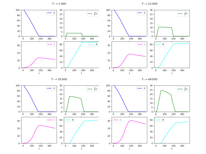
Diagrams of the solutions to (3)–(7)–(8) with a suspension in the vaccination campaign as detailed in (9) in the 4 cases T∗=7,21,35,49
Figure 3.
Diagrams of the solutions to (4)–(7)–(8)–(10). On the left with ω=0.1 and, on the right, with ω=0.4
Figure 4.
Above, the integrations of (1) and (15), below on the left that of (16) (19). The rightmost diagram on the second line displays the total number of living individuals in the three cases, showing that, with respect to mortality, the ODE–PDE model (16) can be seen in some senses in the middle between the ODE models (1) and (15)
Figure 5.
Above, from left to right, the integrations of Case (i), Case (ii) and Case (iii) in (20) with parameters and data as prescribed in (19). Below, the corresponding choices of the ρ function as detailed in (20). The differences in the displayed evolutions are due to the intra–compartmental dynamics in the I population