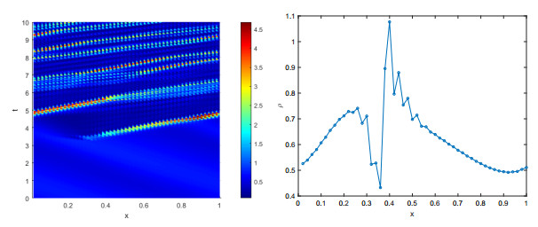
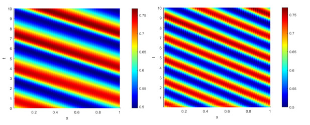
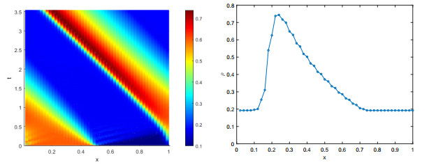
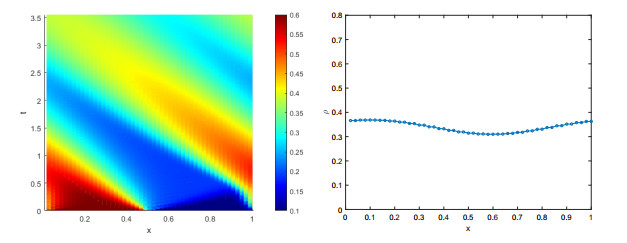
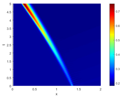
In this article, we investigate theoretical and numerical properties of the first-order Lighthill-Whitham-Richards (LWR) traffic flow model with time delay. Since standard results from the literature are not directly applicable to the delayed model, we mainly focus on the numerical analysis of the proposed finite difference discretization. The simulation results also show that the delay model is able to capture Stop & Go waves.
Citation: Simone Göttlich, Elisa Iacomini, Thomas Jung. Properties of the LWR model with time delay[J]. Networks and Heterogeneous Media, 2021, 16(1): 31-47. doi: 10.3934/nhm.2020032
In this article, we investigate theoretical and numerical properties of the first-order Lighthill-Whitham-Richards (LWR) traffic flow model with time delay. Since standard results from the literature are not directly applicable to the delayed model, we mainly focus on the numerical analysis of the proposed finite difference discretization. The simulation results also show that the delay model is able to capture Stop & Go waves.

| [1] |
Derivation of continuum flow traffic models from microscopic follow-the-leader models. SIAM J. Appl. Math. (2002) 63: 259-278. 
|
| [2] |
Resurrection of "second order" models of traffic flow?. SIAM J. Appl. Math. (2000) 60: 916-938.
|
| [3] | Dynamical model of traffic congestion and numerical simulation. Physical review E (1995) 51: 10-35. |
| [4] |
C. Bianca, M. Ferrara and L. Guerrini, The time delays' effects on the qualitative behavior of an economic growth model, Abstract and Applied Analysis, 2013 (2013). doi: 10.1155/2013/901014
|
| [5] |
Well-posedness of a conservation law with non-local flux arising in traffic flow modeling. Numer. Math. (2016) 132: 217-241.
|
| [6] |
A general phase transition model for vehicular traffic. SIAM Journal on Applied Mathematics (2011) 71: 107-127.
|
| [7] |
A nonlinear discrete velocity relaxation model for traffic flow. SIAM Journal on Applied Mathematics (2018) 78: 2891-2917.
|
| [8] | M. Braskstone and M. McDonald, Car following: A historical review, transportation research part f. 2., Pergamon, 2000. |
| [9] | Derivation of a first order traffic flow model of Lighthill-Whitham-Richards type. IFAC-PapersOnLine (2018) 51: 49-54. |
| [10] |
Derivation of second order traffic flow models with time delays. Netw. Heterog. Media (2019) 14: 265-288.
|
| [11] |
S. Cacace, F. Camilli, R. De Maio and A. Tosin, A measure theoretic approach to traffic flow optimisation on networks, European Journal of Applied Mathematics, (2018), 1-23. doi: 10.1017/S0956792518000621
|
| [12] |
Measure-valued solutions to nonlocal transport equations on networks. Journal of Differential Equations (2018) 264: 7213-7241.
|
| [13] |
Traffic dynamics: Studies in car following. Operations Research (1958) 6: 165-184.
|
| [14] |
Hyperbolic phase transitions in traffic flow. SIAM Journal on Applied Mathematics (2003) 63: 708-721.
|
| [15] |
Non local balance laws in traffic models and crystal growth. ZAMM Z. Angew. Math. Mech. (2007) 87: 449-461.
|
| [16] |
A mixed ode-pde model for vehicular traffic. Mathematical Methods in the Applied Sciences (2015) 38: 1292-1302.
|
| [17] |
R. M. Colombo and E. Rossi, On the micro-macro limit in traffic flow, Rendiconti del Seminario Matematico della Università di Padova, 131 (2014), 217-236. doi: 10.4171/RSMUP/131-13
|
| [18] |
E. Cristiani and E. Iacomini, An interface-free multi-scale multi-order model for traffic flow, Discrete & Continuous Dynamical Systems-Series B, 25 (2019). doi: 10.3934/dcdsb.2019135
|
| [19] |
On the micro-to-macro limit for first-order traffic flow models on networks. Netw. Heterog. Media (2016) 11: 395-413.
|
| [20] | A delay-differential equation model of hiv infection of cd4+ t-cells. Mathematical Biosciences (2000) 165: 27-39. |
| [21] |
Many particle approximation of the Aw-Rascle-Zhang second order model for vehicular traffic. Math. Biosci. Eng. (2017) 14: 127-141.
|
| [22] |
Self-sustained nonlinear waves in traffic flow. Phys. Rev. E (2009) 79: 56-113.
|
| [23] |
A Godunov type scheme for a class of LWR traffic flow models with non-local flux. Netw. Heterog. Media (2018) 13: 531-547.
|
| [24] | M. Garavello and B. Piccoli, Traffic Flow on Networks, AIMS Series on Applied Mathematics, 2006. |
| [25] |
Well-posedness and finite volume approximations of the LWR traffic flow model with non-local velocity. Netw. Heterog. Media (2016) 11: 107-121.
|
| [26] | D. Green Jr. and H. W. Stech, Diffusion and hereditary effects in a class of population models, in Differential Equations and Applications in Ecology, Epidemics, and Population Problems, Elsevier, 1981, 19-28. |
| [27] | B. D. Greenshields, A study in highway capacity, Highway Research Board Proc., 1935, (1935), 448-477. |
| [28] |
The bgk approximation of kinetic models for traffic. Kinetic & Related Models (2020) 13: 279-307.
|
| [29] |
A. Keimer and L. Pflug, Nonlocal conservation laws with time delay, Nonlinear Differential Equations and Applications NoDEA, 26 (2019), 54. doi: 10.1007/s00030-019-0597-z
|
| [30] |
Feedback stabilization of linear systems with delayed control. IEEE Transactions on Automatic control (1980) 25: 266-269.
|
| [31] |
On kinematic waves Ⅱ. A theory of traffic flow on long crowded roads. Proceedings of the Royal Society of London. Series A. Mathematical and Physical Sciences (1955) 229: 317-345.
|
| [32] |
Nonlinear effects in the dynamics of car following. Operations Research (1961) 9: 209-229.
|
| [33] |
B. Piccoli and A. Tosin, Vehicular traffic: A review of continuum mathematical models, in Encyclopedia of Complexity and Systems Science, Springer, New York, NY, 2009, 9727-9749. doi: 10.1007/978-1-4614-1806-1_112
|
| [34] |
G. Puppo, M. Semplice, A. Tosin and G. Visconti, Kinetic models for traffic flow resulting in a reduced space of microscopic velocities, Kinetic & Related Models, 10 (2016), 823. doi: 10.3934/krm.2017033
|
| [35] | A. D. Rey and C. Mackey, Multistability and boundary layer development in a transport equation, Canadian Applied Mathematics Quarterly, (1993), 61-81. |
| [36] |
Shock waves on the highway. Operations Research (1956) 4: 42-51.
|
| [37] | Empirical analysis of the causes of stop-and-go waves at sags. IET Intell. Transp. Syst. (2014) 8: 499-506. |
| [38] |
M. D. Rosini, Macroscopic Models for Vehicular Flows and Crowd Dynamics: Theory and Applications, Understanding Complex Systems, Springer International Publishing, 2013. doi: 10.1007/978-3-319-00155-5
|
| [39] |
H. L. Smith, An Introduction to Delay Differential Equations with Applications to the Life Sciences, 57, Springer, New York, 2011. doi: 10.1007/978-1-4419-7646-8
|
| [40] |
A second order traffic flow model with lane changing. Journal of Scientific Computing (2019) 81: 1429-1445.
|
| [41] | R. E. Stern, et al., Dissipation of stop-and-go waves via control of autonomous vehicles: Field experiments, Transportation Res. Part C, 89 (2018), 205-221. |
| [42] |
From traffic and pedestrian follow-the-leader models with reaction time to first order convection-diffusion flow models. SIAM Journal on Applied Mathematics (2018) 78: 63-79.
|
| [43] | M. Treiber, A. Hennecke and D. Helbing, Derivation, properties, and simulation of a gas-kinetic-based, nonlocal traffic model, Physical Review E, 59 (1999), 239. |
| [44] |
M. Treiber and A. Kesting, Traffic flow dynamics, in Traffic Flow Dynamics: Data, Models and Simulation, Springer-Verlag Berlin Heidelberg, 2013. doi: 10.1007/978-3-642-32460-4
|
| [45] |
Multivalued fundamental diagrams of traffic flow in the kinetic Fokker-Planck limit. Multiscale Model. Simul. (2017) 15: 1267-1293.
|
| [46] | A non-equilibrium traffic model devoid of gas-like behavior. Transportation Research Part B: Methodological (2002) 36: 275-290. |
| [47] | A unified follow-the-leader model for vehicle, bicycle and pedestrian traffic. Transportation Res. Part B (2017) 105: 315-327. |
Figures(9)
Simone Göttlich, Elisa Iacomini, Thomas Jung. Properties of the LWR model with time delay[J]. Networks and Heterogeneous Media, 2021, 16(1): 31-47. doi: 10.3934/nhm.2020032


 DownLoad: